Velocity Model#
For this study we use a modified version of the 3D P- and S-wave velocity model of Delph et al. [2021]. The S-wave velocity model was developed through the joint inversion of adaptive common conversion point-derived P-wave radial receiver functions and Rayleigh wave phase velocity measurements from ambient noise cross correlations following Delph et al. (2015, 2017), and was presented by Delph et al. (2018). To map S-wave velocities to P-wave velocities, Delph et al. [2021] created a 2D crustal Vp/Vs model using Wadati diagrams of earthquakes from the USGS NEIC catalog and low-frequency earthquakes if they were present from Royer & Bostock (2014). These Vp/Vs values were then binned and averaged, and used to convert the 3D crustal S-wave velocities to P-wave velocities as constrained by either the slab top model (McCrory et al. 2012) where the overriding crust lies directly on top of the downgoing slab, or the Moho of the overriding plate. We used a Vp/Vs of 1.78 in the mantle or where no Vp/Vs constraint could be obtained due to lack of earthquakes, as it generally corresponds to the Vp/Vs of peridotite at ~1 GPa as well as intermediate/mafic crust (Christiansen, 1996). The model we use deviates slightly from Delph et al. [2021] in that any S-wave velocities that exceeded 4.5 km/s was automatically set to 4.5 km/s, as expected for uppermost mantle velocities based on global models and laboratory measurements of peridotite (Christensen, 1996; Kennett et al. 1991). Detailed methodologies for creating the S-wave and P-wave velocity model, including the dataset, receiver function computation, and ambient noise methodology, are available in Delph et al. (2018, 2021).
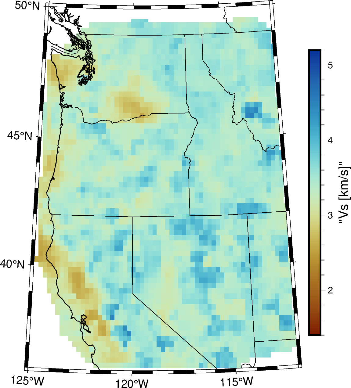
Fig. 3 Delph interpolated velocity model in Cascadia#
In this chapter, you will find 3 notebooks describing the necessary steps to prepare the velocity model into simulPS:
Prepare the polygons json file: helper notebook to write a json file with the necessary parameters to define each area 1_write_poly_param (not necessary to use, it is possible to write the json by hand)
Prepare the velocity model: Convert the 3D velocity to xarray and does the necessary interpolations/extrapolations 2_read_velocity_to_xr
Save the velocity model (P and S) in the simulPS format for all polygons: Takes the json file and the velocity model as input 3_velocity_to_poly_nnl
Generate the NonLinLoc config files to calculate the travel timetables 4_config_file_nll
Run the NonLinLoc commands 5_Vel2Grid2Time_NLLoc
Verify the resulting velocity grids and timetables 6_check_nllgrid