Gridding Cascadia

We use the Eikonal ray tracing software included in nonlinloc to compute travel time tables for the Cascadia Subduction Zone. To keep the grid sizes manageable, we separate Cascadia into 10 subregions that have boundaries that overlap by 0.2\(^\circ\). These subregions are also consistent with the coverage of the Delph et al. velocity model we employ. The lateral dimensions of these grids is <= 245 km which is small enough that the error introduced by using a flat Earth approximation is minimal.

The script grid_locations.py contains the grid names, boundaries, and generates the plot below showing the grid locations.

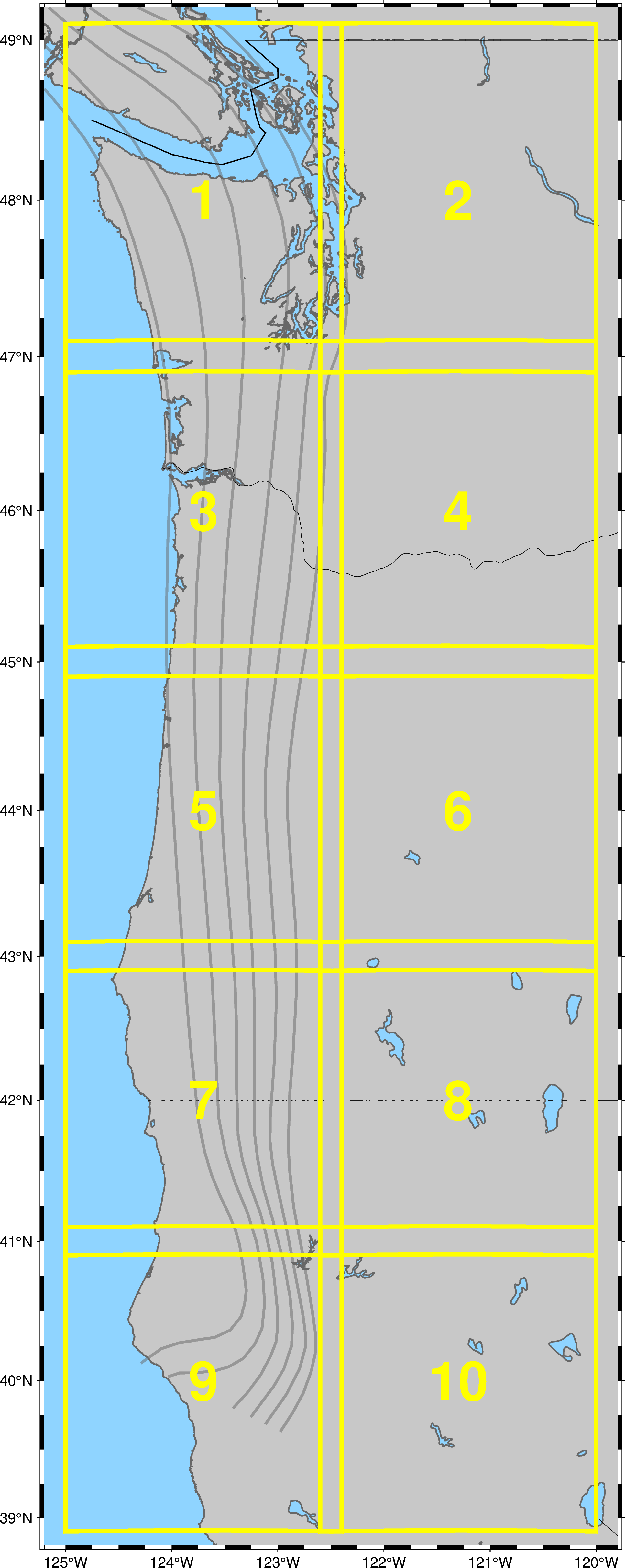
Fig. 4 Velocity model grids in Cascadia

Table 1 Velocity model grid boundaries

Box ID	Minimum Longitude	Maximum Longitude	Minimum Latitude	Maximum Latitude
1	-125	-122.4	46.9	49.1
2	-122.6	-120	46.9	49.1
3	-125	-122.4	44.9	47.1
4	-122.6	-120	44.9	47.1
5	-125	-122.4	42.9	45.1
6	-122.6	-120	42.9	45.1
7	-125	-122.4	40.9	43.1
8	-122.6	-120	40.9	43.1
9	-125	-122.4	38.9	41.1
10	-122.6	-120	38.9	41.1