Prepare velocity model#
Use this notebook to prepare a velocity model as input of the notebook “Velocity_to_poly_nnl”, by doing the necessary interpolations
This notebook might require some adjustments depending on the input velocity model used:
step 1: read and convert velocity to xarray dataset
step 2: vertical extrapolation to have all depth for the available grid points (nearest neighbor interpolation)
step 3: horizontal interpolation ‘cubic’ by depth slice to fill gaps
step 4: save to netcdf
import numpy as np
import pandas as pd
import pygmt
from pyproj import CRS, Transformer
import matplotlib.pyplot as plt
from scipy import interpolate
import xarray as xr
import os
file_path = "../locations/Delphetal2018_1.75VpVs.txt"
df = pd.read_csv(file_path, sep=r'\s+', header=None, names=['lon', 'lat', 'depth', 'Vp', 'Vs'])

# Pivot the DataFrame to get the multi-dimensional array structure
df_pivot = df.pivot_table(index=['lat', 'lon', 'depth'], values=['Vp', 'Vs'])

# Convert the pivoted DataFrame to an xarray Dataset
ds = xr.Dataset.from_dataframe(df_pivot).sel(depth=slice(-4, 100)).reindex({"depth": range(-4, 101)})
ds
<xarray.Dataset> Size: 7MB
Dimensions:  (lat: 68, lon: 65, depth: 105)
Coordinates:
  * lat      (lat) float64 544B 36.0 36.2 36.4 36.6 36.8 ... 48.8 49.0 49.2 49.4
  * lon      (lon) float64 520B -124.8 -124.6 -124.4 ... -112.4 -112.2 -112.0
  * depth    (depth) int64 840B -4 -3 -2 -1 0 1 2 3 ... 93 94 95 96 97 98 99 100
Data variables:
    Vp       (lat, lon, depth) float64 4MB nan nan nan nan ... nan nan nan nan
Vs (lat, lon, depth) float64 4MB nan nan nan nan ... nan nan nan nanvertical interpolation to get velocity between 100km depth and -4km#
ds_interp = ds.interpolate_na(dim="depth", method="nearest", fill_value="extrapolate")
ds_interp
<xarray.Dataset> Size: 7MB
Dimensions:  (lat: 68, lon: 65, depth: 105)
Coordinates:
  * lat      (lat) float64 544B 36.0 36.2 36.4 36.6 36.8 ... 48.8 49.0 49.2 49.4
  * lon      (lon) float64 520B -124.8 -124.6 -124.4 ... -112.4 -112.2 -112.0
  * depth    (depth) int64 840B -4 -3 -2 -1 0 1 2 3 ... 93 94 95 96 97 98 99 100
Data variables:
    Vp       (lat, lon, depth) float64 4MB nan nan nan nan ... nan nan nan nan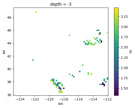
Vs (lat, lon, depth) float64 4MB nan nan nan nan ... nan nan nan nands.sel(depth=-3).Vs.plot()
<matplotlib.collections.QuadMesh at 0x241e925ae10>
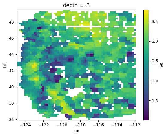
ds_interp.sel(depth=-3).Vs.plot()
<matplotlib.collections.QuadMesh at 0x241ea0085f0>
Interpolation by depth slice to fill gaps#
def interp_depth_slice(depth_data, lon, lat, method='cubic'):
    """
    Interpolates missing data for a specific depth using scipy's griddata.

    Parameters:
    depth_data (np.array): 2D array of data at a specific depth.
    lon (np.array): 1D array of longitudes.
    lat (np.array): 1D array of latitudes.
    method (str): Interpolation method (default is 'cubic').

    Returns:
    np.array: 2D array of interpolated data.
    """
    lon_grid, lat_grid = np.meshgrid(lon, lat)

    # Mask to get the valid data points
    mask = ~np.isnan(depth_data)

    # Coordinates of the valid data points
    points = np.column_stack((lon_grid[mask], lat_grid[mask]))

    # Values of the valid data points
    values = depth_data[mask]

    # Coordinates for the entire grid
    grid_points = np.column_stack((lon_grid.ravel(), lat_grid.ravel()))

    # Perform the interpolation
    interpolated_data = interpolate.griddata(points, values, grid_points, method=method)

    return interpolated_data.reshape(depth_data.shape)

def apply_interpolation(xr_data, method='cubic'):
    """
    Applies interpolation to an xarray DataArray along the depth dimension.

    Parameters:
    xr_data (xr.DataArray): xarray DataArray with dimensions (lon, lat, depth).
    method (str): Interpolation method (default is 'cubic').

    Returns:
    xr.DataArray: Interpolated xarray DataArray.
    """
    # Get the coordinates
    lon = xr_data['lon'].values
    lat = xr_data['lat'].values

    # Use xarray's apply_ufunc to apply the interpolation function to each depth slice
    interpolated = xr.apply_ufunc(
        interp_depth_slice,
        xr_data,
        input_core_dims=[['lat', 'lon']],
        output_core_dims=[['lat', 'lon']],
        vectorize=True,
        dask='parallelized',
        kwargs={'lon': lon, 'lat': lat, 'method': method}
    )

    return interpolated
ds_interp['Vs_interp'] = apply_interpolation(ds_interp.Vs, method='cubic')
ds_interp['Vp_interp'] = apply_interpolation(ds_interp.Vp, method='cubic')
ds_interp
<xarray.Dataset> Size: 15MB
Dimensions:    (lat: 68, lon: 65, depth: 105)
Coordinates:
  * lat        (lat) float64 544B 36.0 36.2 36.4 36.6 ... 48.8 49.0 49.2 49.4
  * lon        (lon) float64 520B -124.8 -124.6 -124.4 ... -112.4 -112.2 -112.0
  * depth      (depth) int64 840B -4 -3 -2 -1 0 1 2 3 ... 94 95 96 97 98 99 100
Data variables:
    Vp         (lat, lon, depth) float64 4MB nan nan nan nan ... nan nan nan nan
    Vs         (lat, lon, depth) float64 4MB nan nan nan nan ... nan nan nan nan
    Vs_interp  (depth, lat, lon) float64 4MB nan nan nan nan ... nan nan nan nan
Vp_interp (depth, lat, lon) float64 4MB nan nan nan nan ... nan nan nan nanverrification plots#
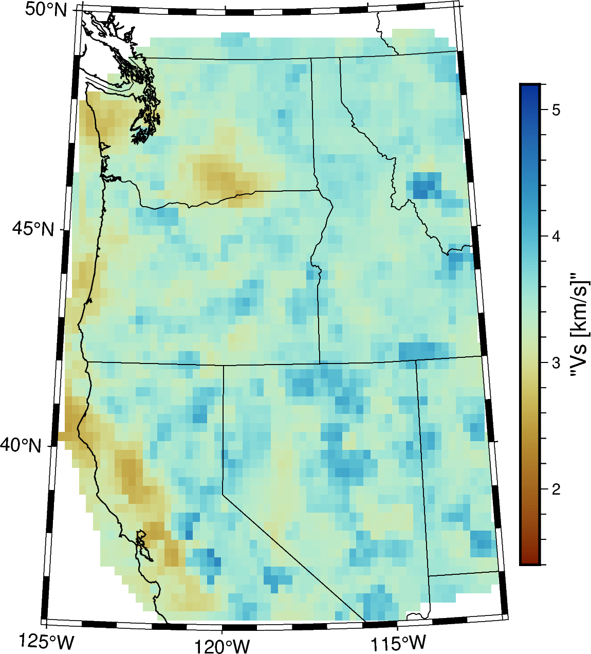
### Example PyGMT Map

# Depth for horizontal slice
depth = 5

# Setting variables related to the colorscale
vmin1 = 1.400
vmax1 = 5.200
vspace = 0.025
vs1_series = (vmin1, vmax1, vspace)
vs1_above = [vmax1,vmax1]
vs1_below = [vmin1,vmin1]

#Setting projection variables
projection = 'L-119.5/37.25/31.5/43/7.5c'
region = [-125,-112,36,50]

# map figure
fig = pygmt.Figure()

# make colormap
pygmt.makecpt(cmap="roma", series=vs1_series)

# Plot a 5km map view slice of the model in isotropic Vs
fig.grdimage(grid=pygmt.grdclip(ds_interp['Vs_interp'].interp(depth = depth, method = "linear"),
                                below=vs1_below, above=vs1_above), projection=projection)
fig.colorbar(frame='af+l"Vs [km/s]"',position="JMR+o0.3c/0c")

# Coast
fig.coast(shorelines = '1/0.5p', region = region, projection=projection,
            frame = ['af'], borders=["1/black", "2/black"])

# stations
#fig.plot(x=sdf["lon"],y=sdf["lat"],style="t1p")

# origin
# fig.plot(x=olon,y=olat,style="c3p",fill="red")

# Show Results
fig.savefig("./velocity_depth5.png", dpi=300)
fig.show()
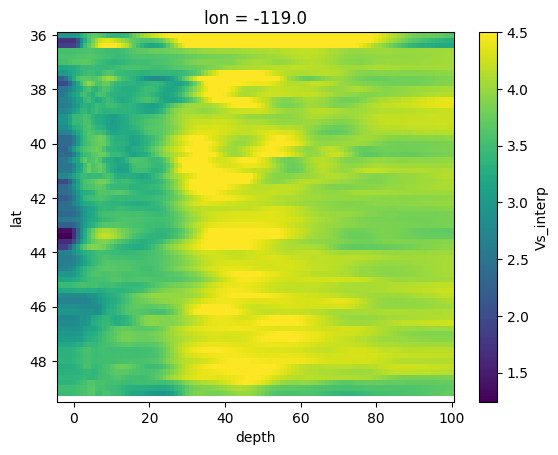
ds_interp.sel(lon=-119).Vs_interp.T.plot()
plt.gca().invert_yaxis()
Save velocity model as netcdf#
ds_interp.to_netcdf("../locations/velocity_interp_delph2018.nc")