Velocity model to polygon simulPS (nnl)

based on Daniel Trugman, 2024 + tips from C. Moody’s analysis notebook
Loïc Bachelot

import numpy as np
import pandas as pd
import pygmt
from pyproj import CRS, Transformer
import matplotlib.pyplot as plt
from scipy import interpolate
import xarray as xr
import os
import json

read json for all polygons to get the input parameters

• Poly id: int

• olat, olon: origin for pyproj projection (center point)

• plat1, plat2: lcc only (min and max of lat)

• xmin, xmax, xsep = -124.0, 124.0, 2.0
  ymin, ymax, ysep = -124.0, 124.0, 2.0
  zmin, zmax, zsep = -4.0, 100.0, 1.0
  cartesian grid bounds for velocity model - must encompass all stations, default values

with open("cascadia_poly.json", 'r+') as file:
    file_data = json.load(file)
file_data[0]

{'poly_id': 1.0,
 'olon': -123.7,
 'olat': 48.0,
 'plat1': 46.9,
 'plat2': 49.1,
 'xmin': -124.0,
 'xmax': 124.0,
 'xsep': 2.0,
 'ymin': -124.0,
 'ymax': 124.0,
 'ysep': 2.0,
 'zmin': -4.0,
 'zmax': 100.0,
 'zsep': 1.0,
 'minlon': -125.0,
 'maxlon': -122.4,
 'minlat': 46.9,
 'maxlat': 49.1}

setup parameter for the selected polygon

### Setup

## Polygon Number: 1-10 and projection
poly = 3
pproj = "lcc" # "tmerc"
maxR = "200R"
print("Polygon", poly)

poly_param = file_data[poly-1]

# origin for pyproj projection
olat, olon = poly_param['olat'], poly_param['olon']

# lcc only
plat1, plat2 = poly_param['plat1'], poly_param['plat2']

# cartesian grid bounds for velocity model
#  - must encompass all stations!
xmin, xmax, xsep = poly_param['xmin'], poly_param['xmax'], poly_param['xsep']
ymin, ymax, ysep = poly_param['ymin'], poly_param['ymax'], poly_param['ysep']
zmin, zmax, zsep = poly_param['zmin'], poly_param['zmax'], poly_param['zsep']

Polygon 3

set output path

# output files
out_dir = "../locations/nlloc3D"
out_fileP = f"{out_dir}/model/delph_simulps_poly{poly}_{pproj}_{maxR}_P.txt"
out_fileS = f"{out_dir}/model/delph_simulps_poly{poly}_{pproj}_{maxR}_S.txt"

Define Projection

# projection setup
crs1 = CRS.from_proj4("+proj=longlat +ellps=WGS84")
if pproj == "lcc":
    crs2 = CRS.from_proj4("+proj={:} +ellps=WGS84 +lat_0={:.4f} +lon_0={:.4f} +lat_1={:.4f} +lon_2={:.4f} +units=km".format(
        pproj,olat,olon,plat1,plat2))
else:
    crs2 = CRS.from_proj4("+proj={:} +ellps=WGS84 +lat_0={:.4f} +lon_0={:.4f} +units=km".format(
        pproj,olat,olon))
proj = Transformer.from_crs(crs1,crs2)
iproj = Transformer.from_crs(crs2,crs1)

Filter datasets and project

load event list

evlist = "../locations/cascadia.earthquakes.filtered"
qdf = pd.read_csv(evlist, parse_dates=['DateTime'])

# filter events for polygon
qdf = qdf[
    (qdf['Longitude'] >= poly_param['minlon']) &
    (qdf['Longitude'] <= poly_param['maxlon']) &
    (qdf['Latitude'] >= poly_param['minlat']) &
    (qdf['Latitude'] <= poly_param['maxlat'])
]

# event bounds
qlon0, qlon1 = qdf["Longitude"].quantile([0,1]).values
qlat0, qlat1 = qdf["Latitude"].quantile([0,1]).values
qlonM, qlatM = (qlon0+qlon1)/2, (qlat0+qlat1)/2
print(qlonM,qlatM)

# projection
qxp, qyp = proj.transform(qdf["Longitude"],qdf["Latitude"])
qdf["X"] = qxp
qdf["Y"] = qyp

# useful for NonLinLoc
print("Projected seismicity bounds:")
print(qdf["X"].min(), qdf["X"].max())
print(qdf["Y"].min(), qdf["Y"].max())

# show results
qdf

-123.69200000000001 46.0004
Projected seismicity bounds:
-98.34504694939974 102.3539043696198
-122.15082088039674 122.8226723669208

	DateTime	Latitude	Longitude	Depth	Magnitude	MagType	EventID	Source	X	Y
39	1970/09/03 03:38:37	46.8973	-123.0958	46.9	2.1	d	10836893	PNSN	46.068818	99.953108
118	1971/05/28 10:42:07	46.5903	-122.4315	14.6	3.4	d	10839063	PNSN	97.250671	66.395792
129	1971/06/16 22:49:32	46.6082	-122.5233	44.5	1.7	d	10839158	PNSN	90.184398	68.280276
185	1971/09/14 13:31:33	46.4772	-122.4320	11.3	2.5	d	10839748	PNSN	97.408813	53.819187
234	1971/12/13 20:59:03	47.0362	-123.4942	27.3	3.6	d	10852228	PNSN	15.652714	115.253177
...	...	...	...	...	...	...	...	...	...	...
194365	2024/06/22 15:05:31	46.5368	-122.4070	24.3	0.3	l	62017716	PNSN	99.223600	60.476475
194374	2024/06/23 03:12:40	46.3553	-122.4153	16.2	2.1	l	62017906	PNSN	98.906146	40.285945
194462	2024/06/28 04:35:24	46.3570	-122.4080	15.1	0.7	l	62011417	PNSN	99.465100	40.483872
194514	2024/07/01 04:21:36	46.1208	-122.4978	18.9	0.7	l	62020301	PNSN	92.941290	14.118270
194515	2024/07/01 04:50:36	46.1232	-122.5025	18.2	1.1	l	62020306	PNSN	92.574026	14.379700

6025 rows × 10 columns

load stations

stlist = "../choosing_stations/cascadia.stations.filtered"

sdf = pd.read_csv(stlist, sep='|', parse_dates=['StartTime', 'EndTime'])
sdf

	Network	Station	Latitude	Longitude	Elevation	Sitename	StartTime	EndTime	Operating_Time
0	BK	DANT	40.294601	-121.802101	967.0	Paynes Creek, CA, USA	2024-06-27 17:40:00	2030-12-31 23:59:59	2378.263877
1	C8	BCOV	50.544200	-126.842700	33.0	Beaver Cove, BC, CA	2020-03-31 00:00:00	2030-12-31 23:59:59	3927.999988
2	C8	BPCB	48.923600	-123.704500	31.0	Bare Point, BC, CA	2008-03-19 00:00:00	2014-06-10 23:59:59	2274.999988
3	C8	FHRB	50.060400	-127.115800	5.0	Fair Harbour, BC, CA	2009-03-12 00:00:00	2015-10-24 23:59:59	2417.999988
4	C8	MWAB	49.741100	-125.303200	1176.0	Mount Washington, BC, CA	2009-07-31 00:00:00	2030-12-31 23:59:59	7823.999988
...	...	...	...	...	...	...	...	...	...
800	CN	VGZ	48.413000	-123.325000	67.0	Victoria Gonzales, BC, CA	1994-07-21 00:00:00	2030-12-31 23:59:59	13312.999988
801	CN	WOSB	50.161000	-126.570000	961.0	Woss, BC, CA	1998-11-17 00:00:00	2030-12-31 23:59:59	11732.999988
802	CN	WPB	49.648000	-123.209000	260.0	Watts Point, BC, CA	1996-09-04 00:00:00	2030-12-31 23:59:59	12536.999988
803	CN	WSLR	50.127000	-122.921000	907.0	Whistler, BC, CA	2003-05-09 00:00:00	2030-12-31 23:59:59	10098.999988
804	CN	YOUB	48.901000	-124.262000	771.0	Youbou Lake Cowichan, BC, CA	2003-02-28 00:00:00	2014-09-03 23:59:59	4205.999988

805 rows × 9 columns

# load all stations
stlist = "../choosing_stations/cascadia.stations.filtered"

sdf = pd.read_csv(stlist, sep='|', parse_dates=['StartTime', 'EndTime'])

# filter stations for polygon
sdf = sdf[
    (sdf['Longitude'] >= poly_param['minlon']) &
    (sdf['Longitude'] <= poly_param['maxlon']) &
    (sdf['Latitude'] >= poly_param['minlat']) &
    (sdf['Latitude'] <= poly_param['maxlat'])
]


# find bounds
slat0, slat1 = sdf["Latitude"].min(), sdf["Latitude"].max()
slon0, slon1 = sdf["Longitude"].min(), sdf["Longitude"].max()
selv0, selv1 = sdf["Elevation"].min(), sdf["Elevation"].max()
print(f"min lon: {slon0}, max lon: {slon1}")
print(f"min lat: {slat0}, max lat: {slat1}")
print(f"min elevation: {selv0}, max elevation: {selv1}")
print()

# center point
slonC, slatC = np.round(0.5*(slon0+slon1),4), np.round(0.5*(slat0+slat1),4)
print(f"Center point lon: {slonC}, lat: {slatC}")
print()

# project coordinates
sxp, syp = proj.transform(sdf["Longitude"], sdf["Latitude"])
sdf["X"] = sxp
sdf["Y"] = syp
print(f"X min: {sdf["X"].min()}, X max: {sdf["X"].max()}")
print(f"Y min: {sdf["Y"].min()}, Y max: {sdf["Y"].max()}")
print()

# check bounds
assert sdf["X"].min() >= xmin
assert sdf["X"].max() <= xmax
assert sdf["Y"].min() >= ymin
assert sdf["Y"].max() <= ymax

# show dataframe
sdf

min lon: -124.07024, max lon: -122.401932
min lat: 45.02753, max lat: 47.08075
min elevation: 5.4, max elevation: 1130.0

Center point lon: -123.2361, lat: 46.0541

X min: -28.27793470777001, X max: 100.44969306512377
Y min: -108.0895647308553, Y max: 120.22042010062447

	Network	Station	Latitude	Longitude	Elevation	Sitename	StartTime	EndTime	Operating_Time	X	Y
20	CC	CC	45.610920	-122.496130	66.66	Rainier Lahar Test Station	2019-01-01	2030-12-31 23:59:59	4382.999988	93.911013	-42.554342
37	CC	HUT1	45.611260	-122.496760	86.00	HUT 1	2023-02-10	2030-12-31 23:59:59	2881.999988	93.861311	-42.517283
54	CC	PR00	45.610920	-122.496130	66.66	Rainier Lahar Test Station	2019-01-01	2030-12-31 23:59:59	4382.999988	93.911013	-42.554342
95	GS	TAUL1	45.522769	-123.054179	56.00	Cornelius Elementary School, Cornelius, OR,USA	2021-05-25	2030-12-31 23:59:59	3507.999988	50.458219	-52.848057
96	GS	TAUL2	45.518911	-123.109937	58.00	Forest Grove Fire Dept, Forest Grove, OR, USA	2021-05-26	2030-12-31 23:59:59	3506.999988	46.105025	-53.310022
...	...	...	...	...	...	...	...	...	...	...	...
525	UW	TOUT	46.303180	-122.563060	821.50	Weyerhaeuser Mt St Helens Tree Farm, Cowlitz C...	2023-06-04	2030-12-31 23:59:59	2767.999988	87.612402	34.321467
546	UW	WHGC	46.655991	-123.729866	5.40	Willapa Harbor Golf Course, WA, USA	2019-02-03	2030-12-31 23:59:59	4349.999988	-2.287108	72.942066
550	UW	WPO	45.572830	-122.790527	335.40	West Portland, OR, USA	1986-10-16	2030-12-31 23:59:59	16147.999988	70.994361	-47.086798
555	UW	YACT	45.932500	-122.419300	214.00	Yacolt, WA, USA	2005-05-10	2030-12-31 23:59:59	9366.999988	99.339867	-6.720267
556	UW	YELM	46.940160	-122.590810	102.90	Yelm Schools Facilities and Maintenance, Yelm,...	2021-11-15	2030-12-31 23:59:59	3333.999988	84.506109	105.126743

91 rows × 11 columns

### Project

# create evenly spaced grid
xgrid, ygrid = np.meshgrid(
    np.arange(xmin,xmax+xsep/2,xsep),
    np.arange(ymin,ymax+ysep/2,ysep))

# print
print(xgrid)
print()
print(ygrid)
print()

# project 
lon_grid, lat_grid = iproj.transform(xgrid,ygrid)

# print
print(lon_grid)
print()
print(lat_grid)

[[-124. -122. -120. ...  120.  122.  124.]
 [-124. -122. -120. ...  120.  122.  124.]
 [-124. -122. -120. ...  120.  122.  124.]
 ...
 [-124. -122. -120. ...  120.  122.  124.]
 [-124. -122. -120. ...  120.  122.  124.]
 [-124. -122. -120. ...  120.  122.  124.]]

[[-124. -124. -124. ... -124. -124. -124.]
 [-122. -122. -122. ... -122. -122. -122.]
 [-120. -120. -120. ... -120. -120. -120.]
 ...
 [ 120.  120.  120. ...  120.  120.  120.]
 [ 122.  122.  122. ...  122.  122.  122.]
 [ 124.  124.  124. ...  124.  124.  124.]]

[[-125.26931988 -125.24401442 -125.21870867 ... -122.18129133
  -122.15598558 -122.13068012]
 [-125.26980934 -125.24449599 -125.21918235 ... -122.18081765
  -122.15550401 -122.13019066]
 [-125.2702991  -125.24497786 -125.21965632 ... -122.18034368
  -122.15502214 -122.1297009 ]
 ...
 [-125.33137539 -125.3050698  -125.27876387 ... -122.12123613
  -122.0949302  -122.06862461]
 [-125.33190432 -125.30559021 -125.27927575 ... -122.12072425
  -122.09440979 -122.06809568]
 [-125.3324336  -125.30611095 -125.27978797 ... -122.12021203
  -122.09388905 -122.0675664 ]]

[[44.87357522 44.87392034 44.87425986 ... 44.87425986 44.87392034
  44.87357522]
 [44.89156888 44.89191411 44.89225373 ... 44.89225373 44.89191411
  44.89156888]
 [44.90956248 44.90990782 44.91024754 ... 44.91024754 44.90990782
  44.90956248]
 ...
 [47.06784496 47.06820333 47.06855588 ... 47.06855588 47.06820333
  47.06784496]
 [47.08581831 47.08617679 47.08652944 ... 47.08652944 47.08617679
  47.08581831]
 [47.10379138 47.10414997 47.10450273 ... 47.10450273 47.10414997
  47.10379138]]

load velocity model

### Load xarray dataset
f_nc = "../locations/velocity_interp_delph2018.nc"
# load 
velocity = xr.open_dataset(f_nc)

# show fields
velocity

<xarray.Dataset> Size: 15MB
Dimensions:    (lat: 68, lon: 65, depth: 105)
Coordinates:
  * lat        (lat) float64 544B 36.0 36.2 36.4 36.6 ... 48.8 49.0 49.2 49.4
  * lon        (lon) float64 520B -124.8 -124.6 -124.4 ... -112.4 -112.2 -112.0
  * depth      (depth) int64 840B -4 -3 -2 -1 0 1 2 3 ... 94 95 96 97 98 99 100
Data variables:
    Vp         (lat, lon, depth) float64 4MB ...
    Vs         (lat, lon, depth) float64 4MB ...
    Vs_interp  (depth, lat, lon) float64 4MB ...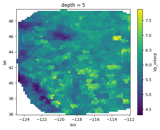
    Vp_interp  (depth, lat, lon) float64 4MB ...

xarray.Dataset

• Dimensions:
  • lat: 68
  • lon: 65
  • depth: 105
• Coordinates: (3)
  • lat
    (lat)
    float64
    36.0 36.2 36.4 ... 49.0 49.2 49.4

    array([36. , 36.2, 36.4, 36.6, 36.8, 37. , 37.2, 37.4, 37.6, 37.8, 38. , 38.2,
           38.4, 38.6, 38.8, 39. , 39.2, 39.4, 39.6, 39.8, 40. , 40.2, 40.4, 40.6,
           40.8, 41. , 41.2, 41.4, 41.6, 41.8, 42. , 42.2, 42.4, 42.6, 42.8, 43. ,
           43.2, 43.4, 43.6, 43.8, 44. , 44.2, 44.4, 44.6, 44.8, 45. , 45.2, 45.4,
           45.6, 45.8, 46. , 46.2, 46.4, 46.6, 46.8, 47. , 47.2, 47.4, 47.6, 47.8,
           48. , 48.2, 48.4, 48.6, 48.8, 49. , 49.2, 49.4])

  • lon
    (lon)
    float64
    -124.8 -124.6 ... -112.2 -112.0

    array([-124.8, -124.6, -124.4, -124.2, -124. , -123.8, -123.6, -123.4, -123.2,
           -123. , -122.8, -122.6, -122.4, -122.2, -122. , -121.8, -121.6, -121.4,
           -121.2, -121. , -120.8, -120.6, -120.4, -120.2, -120. , -119.8, -119.6,
           -119.4, -119.2, -119. , -118.8, -118.6, -118.4, -118.2, -118. , -117.8,
           -117.6, -117.4, -117.2, -117. , -116.8, -116.6, -116.4, -116.2, -116. ,
           -115.8, -115.6, -115.4, -115.2, -115. , -114.8, -114.6, -114.4, -114.2,
           -114. , -113.8, -113.6, -113.4, -113.2, -113. , -112.8, -112.6, -112.4,
           -112.2, -112. ])

  • depth
    (depth)
    int64
    -4 -3 -2 -1 0 1 ... 96 97 98 99 100

    array([ -4,  -3,  -2,  -1,   0,   1,   2,   3,   4,   5,   6,   7,   8,   9,
            10,  11,  12,  13,  14,  15,  16,  17,  18,  19,  20,  21,  22,  23,
            24,  25,  26,  27,  28,  29,  30,  31,  32,  33,  34,  35,  36,  37,
            38,  39,  40,  41,  42,  43,  44,  45,  46,  47,  48,  49,  50,  51,
            52,  53,  54,  55,  56,  57,  58,  59,  60,  61,  62,  63,  64,  65,
            66,  67,  68,  69,  70,  71,  72,  73,  74,  75,  76,  77,  78,  79,
            80,  81,  82,  83,  84,  85,  86,  87,  88,  89,  90,  91,  92,  93,
            94,  95,  96,  97,  98,  99, 100])

• Data variables: (4)
  • Vp
    (lat, lon, depth)
    float64
    ...

    [464100 values with dtype=float64]

  • Vs
    (lat, lon, depth)
    float64
    ...

    [464100 values with dtype=float64]

  • Vs_interp
    (depth, lat, lon)
    float64
    ...

    [464100 values with dtype=float64]

  • Vp_interp
    (depth, lat, lon)
    float64
    ...

    [464100 values with dtype=float64]

• Indexes: (3)
  • lat
    PandasIndex

    PandasIndex(Index([36.0, 36.2, 36.4, 36.6, 36.8, 37.0, 37.2, 37.4, 37.6, 37.8, 38.0, 38.2,
           38.4, 38.6, 38.8, 39.0, 39.2, 39.4, 39.6, 39.8, 40.0, 40.2, 40.4, 40.6,
           40.8, 41.0, 41.2, 41.4, 41.6, 41.8, 42.0, 42.2, 42.4, 42.6, 42.8, 43.0,
           43.2, 43.4, 43.6, 43.8, 44.0, 44.2, 44.4, 44.6, 44.8, 45.0, 45.2, 45.4,
           45.6, 45.8, 46.0, 46.2, 46.4, 46.6, 46.8, 47.0, 47.2, 47.4, 47.6, 47.8,
           48.0, 48.2, 48.4, 48.6, 48.8, 49.0, 49.2, 49.4],
          dtype='float64', name='lat'))

  • lon
    PandasIndex

    PandasIndex(Index([-124.8, -124.6, -124.4, -124.2, -124.0, -123.8, -123.6, -123.4, -123.2,
           -123.0, -122.8, -122.6, -122.4, -122.2, -122.0, -121.8, -121.6, -121.4,
           -121.2, -121.0, -120.8, -120.6, -120.4, -120.2, -120.0, -119.8, -119.6,
           -119.4, -119.2, -119.0, -118.8, -118.6, -118.4, -118.2, -118.0, -117.8,
           -117.6, -117.4, -117.2, -117.0, -116.8, -116.6, -116.4, -116.2, -116.0,
           -115.8, -115.6, -115.4, -115.2, -115.0, -114.8, -114.6, -114.4, -114.2,
           -114.0, -113.8, -113.6, -113.4, -113.2, -113.0, -112.8, -112.6, -112.4,
           -112.2, -112.0],
          dtype='float64', name='lon'))

  • depth
    PandasIndex

    PandasIndex(Index([ -4,  -3,  -2,  -1,   0,   1,   2,   3,   4,   5,
           ...
            91,  92,  93,  94,  95,  96,  97,  98,  99, 100],
          dtype='int64', name='depth', length=105))

• Attributes: (0)

# fixed depth, map view
velocity['Vp_interp'].sel(depth = 5).plot()
plt.show()

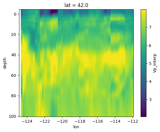
# cross section
velocity['Vp_interp'].sel(lat = 42).plot(y = 'depth')
plt.gca().invert_yaxis()
plt.show()

### Example PyGMT Map

# Depth for horizontal slice
depth = 0

# Setting variables related to the colorscale
vmin1 = 1.400
vmax1 = 5.200
vspace = 0.025
vs1_series = (vmin1, vmax1, vspace)
vs1_above = [vmax1,vmax1]
vs1_below = [vmin1,vmin1]

#Setting projection variables
projection = 'L-118/44/36/49/7.5c'
region = [-125,-112,36,50]

# map figure
fig = pygmt.Figure()

# make colormap
pygmt.makecpt(cmap="roma", series=vs1_series)

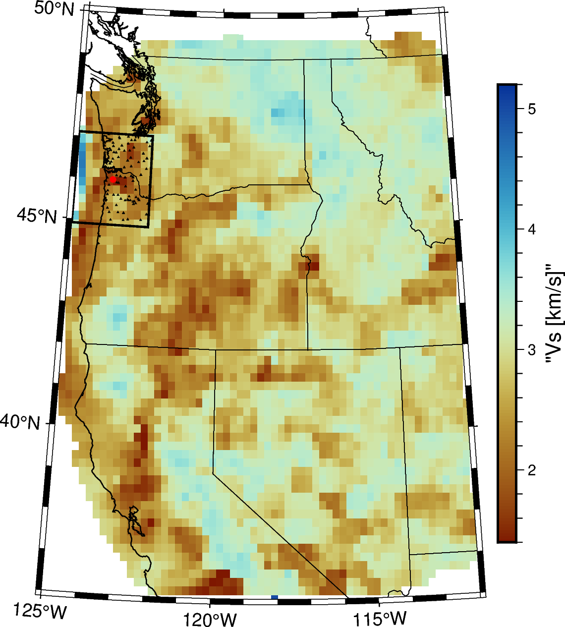
# Plot a 5km map view slice of the model in isotropic Vs
fig.grdimage(grid=pygmt.grdclip(velocity['Vs_interp'].sel(depth=depth), 
                                below=vs1_below, above=vs1_above), projection=projection)
fig.colorbar(frame='af+l"Vs [km/s]"',position="JMR+o0.3c/0c")

# Coast
fig.coast(shorelines = '1/0.5p', region = region, projection=projection,
            frame = ['af'], borders=["1/black", "2/black"])

# stations
fig.plot(x=sdf["Longitude"],y=sdf["Latitude"],style="t1p")

# origin
fig.plot(x=olon,y=olat,style="c3p",fill="red")

# selected polygon
fig.plot(x=[poly_param['minlon'], poly_param['minlon'], poly_param['maxlon'], poly_param['maxlon'], poly_param['minlon']],
         y=[poly_param['minlat'], poly_param['maxlat'], poly_param['maxlat'], poly_param['minlat'], poly_param['minlat']]
        , pen="1p, black")


# Show Results
# fig.savefig("./velocity_depth5.png", dpi=300)
fig.show()

grdinfo [WARNING]: Guessing of registration in conflict between x and y, using gridline

project velocity to polygon

### Compile DataFrame Using Scipy Interpolate
#  - The Xarray version is much slower and crashes...

# first get flattened arrays for output grid
x_flat, y_flat = np.ravel(xgrid), np.ravel(ygrid)
out_lonflat, out_latflat = np.ravel(lon_grid), np.ravel(lat_grid)

# from velocity model
longrid, latgrid = np.meshgrid(
    np.asarray(velocity.lon), np.asarray(velocity.lat))
print(longrid.shape)
vel_lonflat = np.ravel(longrid)
vel_latflat = np.ravel(latgrid)

# 2D arrays as input for scipy.interpolate
out_obs = np.vstack([out_lonflat, out_latflat]).T
vel_obs = np.vstack([vel_lonflat, vel_latflat]).T

# store data here
xvals, yvals, zvals, vpvals, vsvals = [], [], [], [], []

# loop over depths
for zz in np.arange(-4.0, zmax+zsep, zsep): 
    vel_vp = np.ravel(velocity['Vp_interp'].interp(depth = zz, method = 'linear').values)
    vel_vs = np.ravel(velocity['Vs_interp'].interp(depth = zz, method = 'linear').values)
    # interpolation
    out_vp = interpolate.griddata(vel_obs, vel_vp, out_obs, method="linear")
    out_vs = interpolate.griddata(vel_obs, vel_vs, out_obs, method="linear")

    # update
    xvals.append(x_flat)
    yvals.append(y_flat)
    zvals.append(zz + np.zeros(y_flat.size))
    vpvals.append(out_vp) # km/s
    vsvals.append(out_vs) # km/s

    # progress
    if np.mod(zz,10.0) < 0.1: print("Done with depth",zz)

# completed everything
print("Done")

(68, 65)
Done with depth 0.0
Done with depth 10.0
Done with depth 20.0
Done with depth 30.0
Done with depth 40.0
Done with depth 50.0
Done with depth 60.0
Done with depth 70.0
Done with depth 80.0
Done with depth 90.0
Done with depth 100.0
Done

## Turn This Into DataFrame

# make dataframe
odf = pd.DataFrame({
    "x": np.hstack(xvals),
    "y": np.hstack(yvals),
    "z": np.hstack(zvals),
    "vp": np.hstack(vpvals),
    "vs": np.hstack(vsvals),
})

# grid points
xg= odf["x"].unique()
yg = odf["y"].unique()
zg = odf["z"].unique()
nx, ny, nz = len(xg), len(yg), len(zg)
print(nx, ny, nz)

# test groupby z and y
gdf = odf.groupby(["z","y"])
print(gdf.get_group((15.0,-100.0)))

# show 
odf

125 125 105
            x      y     z        vp        vs
298375 -124.0 -100.0  15.0       NaN       NaN
298376 -122.0 -100.0  15.0       NaN       NaN
298377 -120.0 -100.0  15.0       NaN       NaN
298378 -118.0 -100.0  15.0       NaN       NaN
298379 -116.0 -100.0  15.0       NaN       NaN
...       ...    ...   ...       ...       ...
298495  116.0 -100.0  15.0  6.192784  3.538732
298496  118.0 -100.0  15.0  6.195986  3.540562
298497  120.0 -100.0  15.0  6.193055  3.538888
298498  122.0 -100.0  15.0  6.189876  3.537071
298499  124.0 -100.0  15.0  6.186695  3.535254

[125 rows x 5 columns]

	x	y	z	vp	vs
0	-124.0	-124.0	-4.0	NaN	NaN
1	-122.0	-124.0	-4.0	NaN	NaN
2	-120.0	-124.0	-4.0	NaN	NaN
3	-118.0	-124.0	-4.0	NaN	NaN
4	-116.0	-124.0	-4.0	NaN	NaN
...	...	...	...	...	...
1640620	116.0	124.0	100.0	7.325150	4.185799
1640621	118.0	124.0	100.0	7.362251	4.206999
1640622	120.0	124.0	100.0	7.399359	4.228203
1640623	122.0	124.0	100.0	7.434268	4.248152
1640624	124.0	124.0	100.0	7.441389	4.252221

1640625 rows × 5 columns

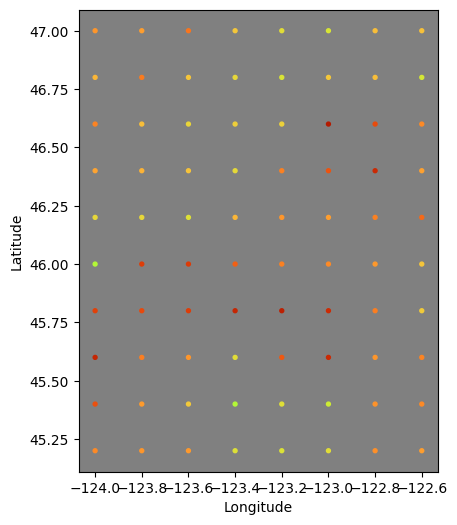
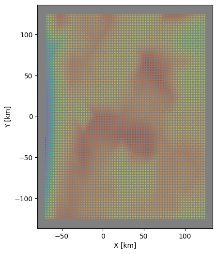
### Test Plot - Notice the Shallow NaN values for interp

test_depth = 0.0


# select data from the xarray
data = velocity["Vs_interp"].interp(depth = test_depth, method = "linear")
vmin = data.min().data
vmax = data.max().data

print(data)
print(f"vmin={vmin}, vmax={vmax}")
lons = np.asarray(data.lon)
lats = np.asarray(data.lat)
mx, my = np.meshgrid(lons,lats)
fx, fy = np.ravel(mx), np.ravel(my)
md = np.ravel(data.values)

# only within the study region bounds
idx = (fx>=slon0)&(fx<=slon1)&(fy>=slat0)&(fy<=slat1)


# plot results to check
fig, axi = plt.subplots(figsize=(6,6))
axi.set_aspect("equal")
axi.set_facecolor("gray")
axi.scatter(fx[idx],fy[idx],s=8,c=md[idx],vmin=vmin,vmax=vmax,
            cmap=plt.cm.turbo_r)
axi.set_xlabel("Longitude")
axi.set_ylabel("Latitude")
plt.show()


# select data from dataframe 
zdf = odf.groupby("z").get_group(test_depth)

# now plot results to check
fig, axi = plt.subplots(figsize=(6,6))
axi.set_aspect("equal")
axi.set_facecolor("gray")
axi.scatter(zdf["x"],zdf["y"],s=0.15,c=zdf["vs"], vmin=vmin, vmax=vmax,
            cmap=plt.cm.turbo_r)
axi.set_xlabel("X [km]")
axi.set_ylabel("Y [km]")
plt.show()

<xarray.DataArray 'Vs_interp' (lat: 68, lon: 65)> Size: 35kB
array([[   nan,    nan,    nan, ...,    nan,    nan,    nan],
       [   nan,    nan,    nan, ...,    nan,    nan,    nan],
       [   nan,    nan,    nan, ...,    nan,    nan,    nan],
       ...,
       [   nan,    nan,    nan, ..., 2.5081,    nan,    nan],
       [   nan,    nan,    nan, ...,    nan,    nan,    nan],
       [   nan,    nan,    nan, ...,    nan,    nan,    nan]])
Coordinates:
  * lat      (lat) float64 544B 36.0 36.2 36.4 36.6 36.8 ... 48.8 49.0 49.2 49.4
  * lon      (lon) float64 520B -124.8 -124.6 -124.4 ... -112.4 -112.2 -112.0
    depth    float64 8B 0.0
vmin=1.0172, vmax=5.138352709337095

fill NaNs

# Function to fill NaN values using nearest neighbors
def fill_nan_with_nearest_neighbors(df, columns):
    for z_val in df['z'].unique():
        subset = df[df['z'] == z_val]
        for col in columns:
            mask = subset[col].notna()
            points = subset[mask][['x', 'y']].values
            values = subset[mask][col].values
            grid = subset[['x', 'y']].values
            filled_values = interpolate.griddata(points, values, grid, method='nearest')
            df.loc[df['z'] == z_val, col] = filled_values
    return df

# Fill NaN values for vp and vs
odf = fill_nan_with_nearest_neighbors(odf, ['vp', 'vs'])
odf

	x	y	z	vp	vs
0	-124.0	-124.0	-4.0	5.967288	3.409882
1	-122.0	-124.0	-4.0	5.967288	3.409882
2	-120.0	-124.0	-4.0	5.967288	3.409882
3	-118.0	-124.0	-4.0	5.967288	3.409882
4	-116.0	-124.0	-4.0	5.967288	3.409882
...	...	...	...	...	...
1640620	116.0	124.0	100.0	7.325150	4.185799
1640621	118.0	124.0	100.0	7.362251	4.206999
1640622	120.0	124.0	100.0	7.399359	4.228203
1640623	122.0	124.0	100.0	7.434268	4.248152
1640624	124.0	124.0	100.0	7.441389	4.252221

1640625 rows × 5 columns

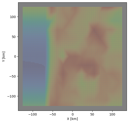
# select data from dataframe 
zdf = odf.groupby("z").get_group(test_depth)

# now plot results to check
fig, axi = plt.subplots(figsize=(6,6))
axi.set_aspect("equal")
axi.set_facecolor("gray")
axi.scatter(zdf["x"],zdf["y"],s=0.15,c=zdf["vs"], vmin=vmin, vmax=vmax,
            cmap=plt.cm.turbo_r)
axi.set_xlabel("X [km]")
axi.set_ylabel("Y [km]")
plt.show()

Save velocity grid

### Write Vp Grid

# open output file
with open(out_fileP,"w") as f:
    
    # header line
    unit, nph = 1.0, 2 # grid units are 1km, 2 phases
    f.writelines("%f %d %d %d %d # SimulPS P-wave Model\n" %(unit,nx,ny,nz,nph))
    
    # write xgrid, ygrid, zgrid
    s = " ".join("%.1f" %x for x in xg) + "\n"
    f.writelines(s)
    s = " ".join("%.1f" %y for y in yg) + "\n"
    f.writelines(s)
    s = " ".join("%.1f" %z for z in zg) + "\n"
    f.writelines(s)
    
    # dummy lines
    f.writelines("0 0 0\n\n")
    
    # loop over z, then y, then write all x
    gdf = odf.groupby(["z","y"])
    for zval in zg:
        for yval in yg:
            df = gdf.get_group((zval,yval))
            vdata = df["vp"].values
            s = " ".join("%.2f" %v for v in vdata) + "\n"
            f.writelines(s)

# write results
print("Done with",out_fileP)

Done with ../locations/nlloc3D/model/delph_simulps_poly3_lcc_200R_P.txt

### Write Vs Grid

# open output file
with open(out_fileS,"w") as f:
    
    # header line
    unit, nph = 1.0, 2 # grid units are 1km, 2 phases
    f.writelines("%f %d %d %d %d # SimulPS S-wave Model\n" %(unit,nx,ny,nz,nph))
    
    # write xgrid, ygrid, zgrid
    s = " ".join("%.1f" %x for x in xg) + "\n"
    f.writelines(s)
    s = " ".join("%.1f" %y for y in yg) + "\n"
    f.writelines(s)
    s = " ".join("%.1f" %z for z in zg) + "\n"
    f.writelines(s)
    
    # dummy lines
    f.writelines("0 0 0\n\n")
    
    # loop over z, then y, then write all x
    gdf = odf.groupby(["z","y"])
    for zval in zg:
        for yval in yg:
            df = gdf.get_group((zval,yval))
            vdata = df["vs"].values
            s = " ".join("%.2f" %v for v in vdata) + "\n"
            f.writelines(s)

# write results
print("Done with",out_fileS)

Done with ../locations/nlloc3D/model/delph_simulps_poly3_lcc_200R_S.txt

print("DONE, Polygon",poly)

DONE, Polygon 3