import pandas as pd
import os
import matplotlib.pyplot as plt
from mpl_toolkits.mplot3d import Axes3D
import seaborn as sns
import cartopy.crs as ccrs
import cartopy.feature as cfeature
Compare new locations with original catalog#
df_PNSN = pd.read_csv("../data/events/cascadia_earthquakes_filtered")
df_PNSN
| DateTime | Latitude | Longitude | Depth | Magnitude | MagType | EventID | Source | |
|---|---|---|---|---|---|---|---|---|
| 0 | 1969/02/14 08:33:36 | 48.9398 | -123.0698 | 52.0 | 4.2 | d | 10835098 | PNSN |
| 1 | 1969/02/28 00:37:04 | 48.0000 | -120.0000 | 18.0 | 2.6 | d | 10835103 | PNSN |
| 2 | 1969/03/20 00:39:12 | 48.0998 | -121.0000 | 18.0 | 3.2 | d | 10835108 | PNSN |
| 3 | 1969/04/12 11:10:30 | 46.9807 | -120.3610 | 15.4 | 2.1 | d | 10835208 | PNSN |
| 4 | 1969/06/11 21:45:08 | 48.7998 | -122.0998 | 33.0 | 3.4 | d | 10835408 | PNSN |
| ... | ... | ... | ... | ... | ... | ... | ... | ... |
| 194517 | 2024/07/01 06:45:27 | 46.9080 | -121.8878 | 5.0 | 0.0 | l | 62020326 | PNSN |
| 194518 | 2024/07/01 12:53:48 | 45.3628 | -121.7063 | -0.5 | 0.6 | l | 62020331 | PNSN |
| 194519 | 2024/07/01 17:19:17 | 48.3517 | -122.1638 | 19.0 | 0.9 | l | 62020406 | PNSN |
| 194520 | 2024/07/01 20:06:37 | 46.7797 | -121.8903 | 9.1 | 1.0 | l | 62020476 | PNSN |
| 194521 | 2024/07/01 22:06:00 | 46.9455 | -121.9388 | 11.7 | 0.3 | l | 62020541 | PNSN |
194522 rows × 8 columns
get NLL located events#
data = []
# Open and read the file
with open("./loc/test_loc.sum.grid0.loc.hyp", 'r') as file:
    eventid = None
    for line in file:
        # Extract the eventid from the PUBLIC_ID line
        if line.startswith('PUBLIC_ID'):
            eventid = int(line.split()[1])

        # Extract the geographic info from the GEOGRAPHIC line
        if line.startswith('GEOGRAPHIC'):
            parts = line.split()
            date_part = f"{parts[2]}/{parts[3]}/{parts[4]}"
            time_part = f"{parts[5]}:{parts[6]}:{parts[7]}"

            # Combine date and time and parse it into a datetime object
            datetime_str = f"{date_part} {time_part}"

            lat = float(parts[9])  # Latitude
            lon = float(parts[11])  # Longitude
            depth = float(parts[13])  # Depth
            source = "NLL"

            # Append the extracted info to the data list
            data.append([eventid, datetime_str, lon, lat, depth, source])

# Create a DataFrame from the extracted data
df_NLL = pd.DataFrame(data, columns=['EventID', 'DateTime', 'Longitude', 'Latitude', 'Depth', 'Source'])
df_NLL['DateTime'] = pd.to_datetime(df_NLL['DateTime'])
df_NLL
| EventID | DateTime | Longitude | Latitude | Depth | Source | |
|---|---|---|---|---|---|---|
| 0 | 61500713 | 2019-07-12 19:04:35.559365 | -121.989034 | 47.865234 | 26.502604 | NLL |
| 1 | 61500718 | 2019-07-15 01:48:25.060547 | -122.012295 | 47.867072 | 27.484375 | NLL |
| 2 | 61500723 | 2019-07-15 04:03:53.680912 | -121.983629 | 47.859721 | 28.263021 | NLL |
| 3 | 61500728 | 2019-07-16 17:32:52.599775 | -122.007392 | 47.870668 | 24.945312 | NLL |
| 4 | 61500743 | 2019-07-16 16:31:57.818746 | -122.010515 | 47.876194 | 24.539062 | NLL |
| 5 | 61500748 | 2019-07-12 11:13:03.095827 | -122.004569 | 47.859198 | 25.723958 | NLL |
| 6 | 61500753 | 2019-07-12 12:01:19.185672 | -122.012164 | 47.857566 | 27.755208 | NLL |
| 7 | 61500758 | 2019-07-12 12:26:46.880081 | -122.012561 | 47.858752 | 27.518229 | NLL |
| 8 | 61500763 | 2019-07-12 12:36:21.546334 | -122.010233 | 47.855598 | 26.028646 | NLL |
| 9 | 61500768 | 2019-07-13 06:40:15.283036 | -121.998090 | 47.858841 | 27.585938 | NLL |
| 10 | 61500773 | 2019-07-13 13:59:11.168556 | -121.990642 | 47.871562 | 25.757812 | NLL |
| 11 | 61500778 | 2019-07-15 00:48:58.114483 | -122.009753 | 47.876199 | 24.268229 | NLL |
| 12 | 61535367 | 2019-07-12 09:53:58.643282 | -122.022452 | 47.857898 | 27.992188 | NLL |
| 13 | 61535372 | 2019-07-12 09:51:37.780540 | -122.043550 | 47.855188 | 26.113281 | NLL |
| 14 | 61535377 | 2019-07-12 09:56:01.965703 | -121.990860 | 47.859281 | 28.703125 | NLL |
| 15 | 61535382 | 2019-07-12 09:59:06.293086 | -122.012208 | 47.860735 | 27.078125 | NLL |
| 16 | 61535397 | 2019-07-12 10:28:56.607880 | -122.001812 | 47.866543 | 26.654948 | NLL |
| 17 | 61535412 | 2019-07-12 10:50:28.767585 | -122.059021 | 47.858454 | 24.132812 | NLL |
| 18 | 61535427 | 2019-07-12 11:24:36.997245 | -121.983702 | 47.865266 | 26.976562 | NLL |
| 19 | 61535432 | 2019-07-12 11:45:37.542329 | -121.986739 | 47.864456 | 28.940104 | NLL |
| 20 | 61535447 | 2019-07-12 12:42:54.170009 | -122.001394 | 47.877835 | 22.914062 | NLL |
| 21 | 61535452 | 2019-07-12 13:00:00.398775 | -122.002746 | 47.865151 | 26.299479 | NLL |
| 22 | 61535477 | 2019-07-12 14:12:39.999586 | -122.018654 | 47.858714 | 29.278646 | NLL |
| 23 | 61535497 | 2019-07-12 15:06:40.268495 | -121.982805 | 47.854972 | 26.367188 | NLL |
| 24 | 61535632 | 2019-07-12 19:20:09.901988 | -122.004162 | 47.857220 | 26.976562 | NLL |
| 25 | 61535657 | 2019-07-12 20:24:52.425056 | -121.997414 | 47.865183 | 26.028646 | NLL |
| 26 | 61535687 | 2019-07-12 21:31:03.171690 | -122.006548 | 47.850669 | 27.162760 | NLL |
| 27 | 61535812 | 2019-07-13 15:04:42.088614 | -122.016209 | 47.860908 | 27.941406 | NLL |
| 28 | 61536017 | 2019-07-14 14:18:41.701378 | -122.046995 | 47.869624 | 27.856771 | NLL |
| 29 | 61536062 | 2019-07-14 17:44:44.379513 | -122.039856 | 47.849864 | 28.466146 | NLL |
| 30 | 61536122 | 2019-07-15 02:30:34.746135 | -122.017816 | 47.853174 | 26.705729 | NLL |
| 31 | 61536131 | 2019-07-16 07:46:44.677659 | -121.998547 | 47.850322 | 26.993490 | NLL |
| 32 | 61536136 | 2019-07-16 09:09:36.330659 | -122.019394 | 47.857125 | 26.773438 | NLL |
| 33 | 61536697 | 2019-07-17 23:43:16.887956 | -122.046790 | 47.855365 | 24.200521 | NLL |
| 34 | 61536812 | 2019-07-18 04:04:34.109631 | -122.024737 | 47.857884 | 26.164062 | NLL |
| 35 | 61537187 | 2019-07-18 23:38:12.940683 | -122.005706 | 47.858795 | 26.231771 | NLL |
Merge both dataframes#
df_PNSP_filtered = df_PNSN[df_PNSN['EventID'].isin(df_NLL['EventID'])]
df_combined = pd.concat([df_PNSP_filtered, df_NLL], ignore_index=True)
df_combined
| DateTime | Latitude | Longitude | Depth | Magnitude | MagType | EventID | Source | |
|---|---|---|---|---|---|---|---|---|
| 0 | 2019/07/12 09:51:38 | 47.872300 | -122.013800 | 29.000000 | 4.6 | l | 61535372 | PNSN |
| 1 | 2019/07/12 09:53:58 | 47.864500 | -122.026200 | 30.800000 | 3.4 | l | 61535367 | PNSN |
| 2 | 2019/07/12 09:56:02 | 47.855300 | -122.036000 | 27.900000 | 1.8 | l | 61535377 | PNSN |
| 3 | 2019/07/12 09:59:06 | 47.862800 | -122.025500 | 27.400000 | 0.9 | d | 61535382 | PNSN |
| 4 | 2019/07/12 10:28:57 | 47.854800 | -122.042800 | 26.000000 | 1.6 | l | 61535397 | PNSN |
| ... | ... | ... | ... | ... | ... | ... | ... | ... |
| 67 | 2019-07-16 07:46:44.677659 | 47.850322 | -121.998547 | 26.993490 | NaN | NaN | 61536131 | NLL |
| 68 | 2019-07-16 09:09:36.330659 | 47.857125 | -122.019394 | 26.773438 | NaN | NaN | 61536136 | NLL |
| 69 | 2019-07-17 23:43:16.887956 | 47.855365 | -122.046790 | 24.200521 | NaN | NaN | 61536697 | NLL |
| 70 | 2019-07-18 04:04:34.109631 | 47.857884 | -122.024737 | 26.164062 | NaN | NaN | 61536812 | NLL |
| 71 | 2019-07-18 23:38:12.940683 | 47.858795 | -122.005706 | 26.231771 | NaN | NaN | 61537187 | NLL |
72 rows × 8 columns
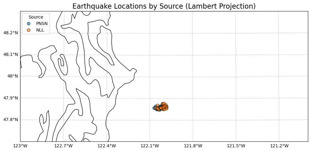
Look on a map#
# Create a figure with a specific size and set Lambert Conformal projection
fig, ax = plt.subplots(figsize=(12, 8), subplot_kw={'projection': ccrs.AlbersEqualArea(central_longitude=-122, central_latitude=48)})

# Add features to the map
ax.add_feature(cfeature.COASTLINE)
ax.add_feature(cfeature.BORDERS, linestyle=':')
ax.add_feature(cfeature.LAKES, facecolor='lightblue')
ax.add_feature(cfeature.RIVERS)

# Set the extent of the map: [west, east, south, north]
ax.set_extent([-123, -121, 47.7, 48.3])

# Plot the data
for source in df_combined['Source'].unique():
    source_data = df_combined[df_combined['Source'] == source]
    ax.scatter(
        source_data['Longitude'],
        source_data['Latitude'],
        label=source,
        s=50,  # Marker size
        alpha=0.6,  # Transparency
        edgecolor='black',  # Edge color for markers
        transform=ccrs.PlateCarree()  # Ensure data is projected correctly
    )

gl = ax.gridlines(draw_labels=True, linewidth=0.5, color='gray', alpha=0.7, linestyle='--', transform=ccrs.PlateCarree())
gl.top_labels = False
gl.right_labels = False
gl.rotate_labels = False

# Add longitude and latitude labels
ax.set_xlabel('Longitude', fontsize=12)
ax.set_ylabel('Latitude', fontsize=12)

# Add title and legend
ax.set_title('Earthquake Locations by Source (Lambert Projection)', fontsize=16)
ax.legend(title='Source', loc='upper left')

# Show the plot
plt.show()
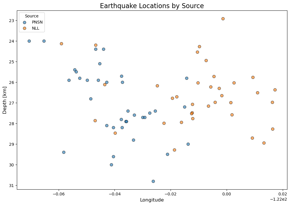
# depth slice along lat
# Create a figure with a specific size and set Lambert Conformal projection
fig, ax = plt.subplots(figsize=(12, 8))

# Plot the data
for source in df_combined['Source'].unique():
    source_data = df_combined[df_combined['Source'] == source]
    ax.scatter(
        source_data['Longitude'],
        source_data['Depth'],
        label=source,
        s=50,  # Marker size
        alpha=0.6,  # Transparency
        edgecolor='black'  # Edge color for markers
    )

# Add longitude and latitude labels
ax.set_xlabel('Longitude', fontsize=12)
ax.set_ylabel('Depth [km]', fontsize=12)
ax.invert_yaxis()
# Add title and legend
ax.set_title('Earthquake Locations by Source', fontsize=16)
ax.legend(title='Source', loc='upper left')

# Show the plot
plt.show()
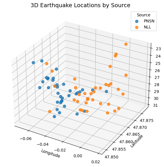
# Set up the figure and the 3D axis
fig = plt.figure(figsize=(10, 7))
ax = fig.add_subplot(111, projection='3d')

# Plot the 3D scatter plot
for i, source in enumerate(df_combined['Source'].unique()):
    source_data = df_combined[df_combined['Source'] == source]
    ax.scatter(
        source_data['Longitude'],  # x-axis
        source_data['Latitude'],   # y-axis
        source_data['Depth'],      # z-axis
        label=source,
        s=50,   # Marker size
        depthshade=True,
        alpha=0.8
    )

# Add axis labels
ax.set_xlabel('Longitude')
ax.set_ylabel('Latitude')
ax.set_zlabel('Depth')

# Invert Z-axis so depth increases downward
ax.invert_zaxis()

# Add legend for Source
ax.legend(title='Source')

# Set plot title
ax.set_title('3D Earthquake Locations by Source', fontsize=14)

# Show the plot
plt.show()