IRIS Web Services Data Quality Metrics Exercise

IRIS Web Services Data Quality Metrics Exercise#

:auth: Nate Stevens (Pacific Northwest Seismic Network) :email: ntsteven@uw.edu
:org: Pacific Northwest Seismic Network
:license: GPLv3
:purpose:
In this notebook we’ll query data quality metrics from the MUSTANG measurements webservice
and the FDSNWS availability webservice provided by EarthScope/SAGE to get a sense of data
availability and usefullness BEFORE downloading a ton of data!

What is MUSTANG? - A continually growing data quality statistics dataset
for every seismic station stored on the Data Management Center!

What does MUSTANG stand for? - The Modular Utility for STAtistical kNowldege Gathering system

Where can I go to learn more about MUSTANG? https://service.iris.edu/mustang/

Dependencies for this Notebook:

ObsPy
ws_client (ws_client.py)

## IMPORT MODULES
import os
from pathlib import Path
import pandas as pd
from obspy import UTCDateTime
from obspy.clients.fdsn import Client
# Tools for data visualization
import matplotlib.pyplot as plt

# Custom-Built Clients for fetching data quality measurements from IRIS web services
from ws_client import MustangClient, AvailabilityClient

# Define absolute paths
ROOT = Path.cwd()
print(f'ROOT dir is {ROOT}')
WFQC = ROOT/'wave_qc_files'
os.makedirs(str(WFQC), exist_ok=True)

ROOT dir is /Users/nates/Code/GitHub/2025_ML_TSC/notebooks/Nate

Composing a MUSTANG query#

The MustangClient class’ get_metrics follows the key=value syntax of the MUSTANG measurements service interface
(https://service.iris.edu/mustang/measurements/1/)
where multiple values can be provided as a comma-delimited string.

This version of the MustangClient can also parse lists of metric names (see below).

The full list of MUSTANG metrics and detailed descriptions of their meaning can be found at the link above.

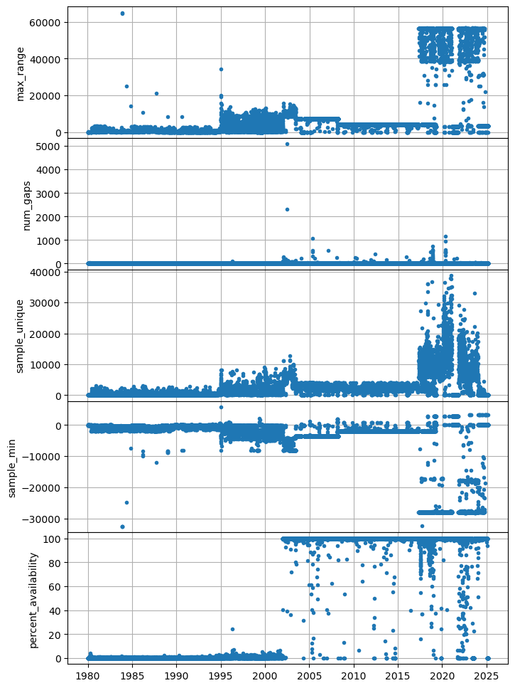
The metrics we’ll use in this exercise are:

sample_min: the minimum sample value observed in a 24 hour period
max_range: the maximum range between any two samples in a 5 minute window within a 24 hour period
percent_availability: the percent of a 24 hour period for which there are data
sample_unique: number of unique sample values reported in a 24 hour window
num_gaps: number of data gaps encountered within a 24 hour window

The seismic station we’re looking at is UW.MBW.01.EHZ, one of the longest running stations in the PNSN that
monitored Mount Baker volcano until late 2023 when it was replaced with UW.MBW2.

UW.MBW was having some issues towards the end of its life, can you find spots where it looks like the data might not be as useful?#

# Initialize the client
mclient = MustangClient()
# Compose a query for MUSTANG metrics for an analog seismometer near Mount Baker (Washington, USA)
metric = ['sample_min','max_range','percent_availability','sample_unique','num_gaps']
query = {'metric': metric,
            'net':'UW',
            'sta':'MBW',
            'loc':'*',
            'cha':'EHZ'}
# Run query (sometimes this requires a few start/stops - something to do with `requests` internal workings)
df_m = mclient.measurements_request(**query)
# Write to disk ()
df_m.to_csv(WFQC/'UW.MBW_MUSTANG_metrics.csv', header=True, index=True)

# Just in case we need to load from disk because `requests` is struggling
try:
    display(df_m)
except NameError:
    df_m = pd.read_csv(WFQC/'UW.MBW_MUSTANG_metrics.csv', index_col=['start','target'], parse_dates=['start'])
    display(df_m)

		max_range	num_gaps	sample_unique	sample_min	percent_availability
start	target
2025-02-11	UW.MBW.01.EHZ.M	3399.0	3.0	22.0	0.0	94.203
2025-02-10	UW.MBW.01.EHZ.M	3380.0	3.0	27.0	0.0	99.985
2025-02-09	UW.MBW.01.EHZ.M	3379.0	3.0	14.0	0.0	99.739
2025-02-08	UW.MBW.01.EHZ.M	3381.0	3.0	17.0	0.0	99.993
2025-02-07	UW.MBW.01.EHZ.M	3394.0	6.0	23.0	0.0	99.990
...	...	...	...	...	...	...
1987-03-20	UW.MBW..EHZ.M	NaN	NaN	NaN	NaN	0.000
1987-01-16	UW.MBW..EHZ.M	NaN	NaN	NaN	NaN	0.000
1987-01-14	UW.MBW..EHZ.M	NaN	NaN	NaN	NaN	0.000
1987-01-26	UW.MBW..EHZ.M	NaN	NaN	NaN	NaN	0.000
1987-01-27	UW.MBW..EHZ.M	NaN	NaN	NaN	NaN	0.000

17093 rows × 5 columns

fig = plt.figure(figsize=(8,12))
gs = fig.add_gridspec(nrows=len(df_m.columns), hspace=0)

for _e, _c in enumerate(df_m.columns):
    ax = fig.add_subplot(gs[_e])
    ax.plot(df_m.index.get_level_values(0), df_m[_c].values, '.', label=_c)
    ax.set_ylabel(_c)
    ax.grid()

../../_images/c0d5c3672ca6ebaecd9557e6bebf2fe44c5cfba3ccd0e600e03b61927a201c01.png

Lots of gaps#

Trying to bulk download gappy data from webservices can result in the entire request crashing.

If we can request with information on data availability (and which data seem to have meaning) then this job becomes easier.

Thankfully data availability is already documented by the NSF SAGE Facility FDSN Web Service!

Running a FDSN Web Service query#

Use the custom-built AvailabilityClient class that follows the syntax of the
related webservice: https://service.iris.edu/fdsnws/availability/1/

For this example we’ll keep looking at station UW.MBW.

# Initialize the client
aclient = AvailabilityClient()
# Run a data availability request for everything UW.MBW.*.EHZ has to offer
df_a = aclient.availability_request(sta='MBW',net='UW',cha='EHZ')
# Write to disk
df_a.to_csv(WFQC/'UW.MBW_Availability.csv', header=True, index=True)

# Take a look at the query results (and an option to read from disk for exercise expediancy)
try:
    display(df_a)
except NameError:
    df_m = pd.read_csv(WFQC/'UW.MBW_Availability.csv', index_col=[0], parse_dates=['Earliest','Latest'])
    display(df_a)

	Network	Station	Location	Channel	Quality	SampleRate	Earliest	Latest
0	UW	MBW		EHZ	M	104.082	1980-01-11 21:40:16.543800+00:00	1980-01-11 21:41:08.185791+00:00
1	UW	MBW		EHZ	M	104.084	1980-01-15 05:34:14.273800+00:00	1980-01-15 05:34:53.617023+00:00
2	UW	MBW		EHZ	M	104.079	1980-01-17 05:39:19.142000+00:00	1980-01-17 05:40:03.406475+00:00
3	UW	MBW		EHZ	M	104.082	1980-01-25 22:40:03.229300+00:00	1980-01-25 22:40:54.871291+00:00
4	UW	MBW		EHZ	M	104.069	1980-01-27 23:41:48.775700+00:00	1980-01-27 23:42:15.825070+00:00
...	...	...	...	...	...	...	...	...
91602	UW	MBW	01	EHZ	M	100.000	2025-02-10 08:00:03+00:00	2025-02-10 08:00:03.990000+00:00
91603	UW	MBW	01	EHZ	M	100.000	2025-02-10 08:00:04.200000+00:00	2025-02-10 08:00:33.190000+00:00
91604	UW	MBW	01	EHZ	M	100.000	2025-02-10 08:00:45.400000+00:00	2025-02-11 08:00:01.390000+00:00
91605	UW	MBW	01	EHZ	M	100.000	2025-02-11 08:00:06.100000+00:00	2025-02-11 08:01:02.090000+00:00
91606	UW	MBW	01	EHZ	M	100.000	2025-02-11 08:01:03+00:00	2025-02-11 22:36:36.990000+00:00

91607 rows × 8 columns

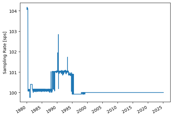
What is going on with the sampling rates?#

_series = pd.Series(df_a.SampleRate.values, index=df_a.Earliest.values)
ax = _series.plot()
ax.set_ylabel('Sampling Rate [sps]')

Text(0, 0.5, 'Sampling Rate [sps]')

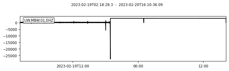
../../_images/3c2c4c0df2d97ee2ccf61400837f16f1e0c08ee27751edebd7b88d6e15fbe379.png

Now lets’ finally look at some data!#

# Get an obspy client for fetching waveforms
wclient = Client('IRIS')

# Subset available segments to a time window (currently uses pandas Timestamp objects)
_df_a = df_a[(df_a.Earliest >= pd.Timestamp('2023-02-19',tz='UTC')) & (df_a.Latest <= pd.Timestamp('2023-02-21',tz='UTC'))]
display(_df_a)

	Network	Station	Location	Channel	Quality	SampleRate	Earliest	Latest
86172	UW	MBW	01	EHZ	M	100.0	2023-02-19 02:18:28.300000+00:00	2023-02-19 02:19:31.290000+00:00
86173	UW	MBW	01	EHZ	M	100.0	2023-02-19 02:19:32.400000+00:00	2023-02-19 08:00:02.390000+00:00
86174	UW	MBW	01	EHZ	M	100.0	2023-02-19 08:00:06.300000+00:00	2023-02-19 12:01:02.290000+00:00
86175	UW	MBW	01	EHZ	M	100.0	2023-02-19 12:01:03.200000+00:00	2023-02-20 01:02:49.190000+00:00
86176	UW	MBW	01	EHZ	M	100.0	2023-02-20 01:02:50.100000+00:00	2023-02-20 02:45:06.090000+00:00
86177	UW	MBW	01	EHZ	M	100.0	2023-02-20 02:45:06.200000+00:00	2023-02-20 02:46:26.190000+00:00
86178	UW	MBW	01	EHZ	M	100.0	2023-02-20 02:46:27.200000+00:00	2023-02-20 08:00:01.190000+00:00
86179	UW	MBW	01	EHZ	M	100.0	2023-02-20 08:00:05.800000+00:00	2023-02-20 08:00:43.790000+00:00
86180	UW	MBW	01	EHZ	M	100.0	2023-02-20 08:00:43.900000+00:00	2023-02-20 11:02:01.890000+00:00
86181	UW	MBW	01	EHZ	M	100.0	2023-02-20 11:05:19.900000+00:00	2023-02-20 13:40:36.890000+00:00
86182	UW	MBW	01	EHZ	M	100.0	2023-02-20 13:40:37+00:00	2023-02-20 13:42:52.990000+00:00
86183	UW	MBW	01	EHZ	M	100.0	2023-02-20 13:42:53.100000+00:00	2023-02-20 16:10:36.090000+00:00

# Compose a bulk request
bulk = []
for _, row in _df_a.iterrows():
    # Switch pandas Timestamp objects back to UTCDateTime objects for requests
    req = (row.Network, row.Station, row.Location, row.Channel, UTCDateTime(row.Earliest.timestamp()), UTCDateTime(row.Latest.timestamp()))
    bulk.append(req)
display(bulk)

[('UW',
  'MBW',
  '01',
  'EHZ',
  2023-02-19T02:18:28.300000Z,
  2023-02-19T02:19:31.290000Z),
 ('UW',
  'MBW',
  '01',
  'EHZ',
  2023-02-19T02:19:32.400000Z,
  2023-02-19T08:00:02.390000Z),
 ('UW',
  'MBW',
  '01',
  'EHZ',
  2023-02-19T08:00:06.300000Z,
  2023-02-19T12:01:02.290000Z),
 ('UW',
  'MBW',
  '01',
  'EHZ',
  2023-02-19T12:01:03.200000Z,
  2023-02-20T01:02:49.190000Z),
 ('UW',
  'MBW',
  '01',
  'EHZ',
  2023-02-20T01:02:50.100000Z,
  2023-02-20T02:45:06.090000Z),
 ('UW',
  'MBW',
  '01',
  'EHZ',
  2023-02-20T02:45:06.200000Z,
  2023-02-20T02:46:26.190000Z),
 ('UW',
  'MBW',
  '01',
  'EHZ',
  2023-02-20T02:46:27.200000Z,
  2023-02-20T08:00:01.190000Z),
 ('UW',
  'MBW',
  '01',
  'EHZ',
  2023-02-20T08:00:05.800000Z,
  2023-02-20T08:00:43.790000Z),
 ('UW',
  'MBW',
  '01',
  'EHZ',
  2023-02-20T08:00:43.900000Z,
  2023-02-20T11:02:01.890000Z),
 ('UW',
  'MBW',
  '01',
  'EHZ',
  2023-02-20T11:05:19.900000Z,
  2023-02-20T13:40:36.890000Z),
 ('UW',
  'MBW',
  '01',
  'EHZ',
  2023-02-20T13:40:37.000000Z,
  2023-02-20T13:42:52.990000Z),
 ('UW',
  'MBW',
  '01',
  'EHZ',
  2023-02-20T13:42:53.100000Z,
  2023-02-20T16:10:36.090000Z)]

# Run bulk request
st = wclient.get_waveforms_bulk(bulk)
st.plot()

../../_images/b0727544efb56e98aadbe096dd6a8217822f3643ec6c11d23ffb0ddb0b715039.png

IRIS Web Services Data Quality Metrics Exercise

Contents

IRIS Web Services Data Quality Metrics Exercise#

Composing a MUSTANG query#

UW.MBW was having some issues towards the end of its life, can you find spots where it looks like the data might not be as useful?#

Lots of gaps#

Running a FDSN Web Service query#

What is going on with the sampling rates?#

Now lets’ finally look at some data!#

It looks like we have continuous data…#

Are they continuous?#

Where do they stop being useful?#

What does this mean for your workflow?#