Double Different Relocation

This notebook will take the phase picks from the associated picks, perform double difference relocation, and plot the earthquake catalog.

by Felix Waldhauser

1. Compute differential times from phase file

%cd /app/hypodd/results_hypodd
%pwd
!ph2dt ph2dt.inp

2. Run double-difference relocation

!hypoDD hypoDD.inp

3. Manipulate the new catalog

import pandas as pd
import matplotlib.pyplot as plt
import numpy as np

Read the relocated catalog

events_hypodd = pd.read_csv('./hypoDD.reloc',header=None, sep="\s+",names=['ID', 'LAT', 'LON', 'DEPTH', 'X', 'Y', 'Z', 'EX', 'EY', 'EZ', 'YR', 'MO', 'DY', 'HR', 'MI', 'SC', 'MAG', 'NCCP', 'NCCS', 'NCTP', 'NCTS', 'RCC', 'RCT', 'CID'])
events_hypodd

	ID	LAT	LON	DEPTH	X	Y	Z	EX	EY	EZ	...	MI	SC	MAG	NCCP	NCCS	NCTP	NCTS	RCC	RCT	CID
0	10	40.479472	-124.313924	17.746	-7130.8	-7587.8	-504.3	495.2	464.1	446.2	...	19	14.89	0.19	0	0	55	51	-9.0	0.140	1
1	13	40.406616	-124.365373	14.527	-11497.3	-15678.1	-3723.3	690.2	1026.9	762.1	...	29	21.75	0.73	0	0	12	4	-9.0	0.150	1
2	14	40.514408	-124.419613	15.401	-16083.8	-3708.3	-2849.4	192.7	270.9	159.0	...	34	24.66	6.09	0	0	654	711	-9.0	0.211	1
3	15	40.588436	-124.114697	17.217	9745.9	4512.1	-1033.3	140.1	208.6	287.0	...	35	59.17	3.73	0	0	604	798	-9.0	0.168	1
4	16	40.517322	-124.329557	17.127	-8453.4	-3384.8	-1123.4	194.0	236.8	165.0	...	36	14.62	3.13	0	0	156	443	-9.0	0.109	1
...	...	...	...	...	...	...	...	...	...	...	...	...	...	...	...	...	...	...	...	...	...
1050	1157	40.539779	-123.959904	19.063	22862.3	-891.0	812.6	255.0	327.8	480.5	...	54	8.52	0.57	0	0	446	560	-9.0	0.167	1
1051	1158	40.576978	-124.399479	22.143	-14371.3	3239.7	3892.7	572.0	520.1	569.1	...	55	52.26	0.75	0	0	11	9	-9.0	0.188	1
1052	1159	40.531274	-124.299154	15.873	-5876.8	-1835.4	-2377.1	308.1	240.9	309.0	...	56	37.56	0.74	0	0	232	293	-9.0	0.175	1
1053	1160	40.633927	-123.987695	19.623	20493.8	9563.7	1372.9	192.8	278.0	307.1	...	58	40.20	1.13	0	0	370	412	-9.0	0.179	1
1054	1161	40.628231	-124.004533	17.401	19069.2	8931.2	-849.6	186.2	260.1	280.6	...	59	34.48	0.62	0	0	190	217	-9.0	0.188	1

1055 rows × 24 columns

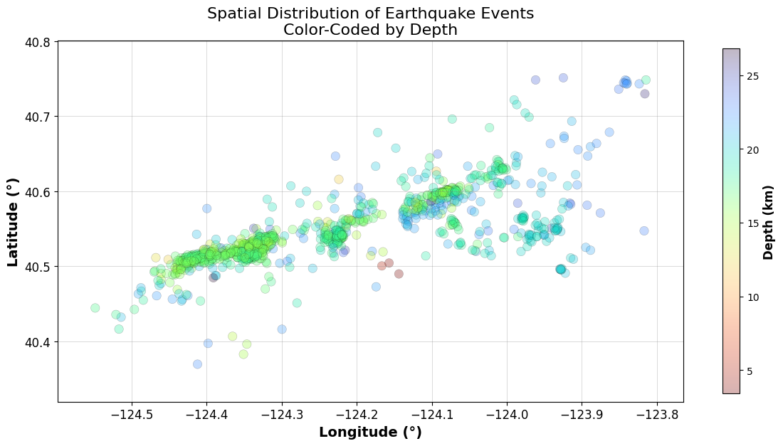
Plot

# Create a figure for the plot
fig = plt.figure(figsize=(12, 10))
ax = fig.add_subplot(111)

# Create scatter plot with depth-coded colors
scatter = ax.scatter(events_hypodd['LON'], events_hypodd['LAT'], 
                    c=events_hypodd['DEPTH'],
                    cmap='turbo_r',  # Use reversed turbo colormap (red for deep, blue for shallow)
                    s=80,  # marker size for good visibility
                    marker='o',
                    edgecolor='k',
                    linewidth=0.3,
                    alpha=0.3)

# Add colorbar with depth information
cbar = plt.colorbar(scatter, ax=ax, shrink=0.5)  # Adjust shrink to make the colorbar smaller
cbar.set_label('Depth (km)', fontsize=12, fontweight='bold')
cbar.ax.tick_params(labelsize=10)

# Set equal aspect ratio for proper geographical representation
ax.set_aspect('equal')

# Add grid with crisp styling
ax.grid(True, linestyle='-', linewidth=0.5, alpha=0.4, color='gray')

# Add descriptive labels
ax.set_xlabel('Longitude (°)', fontsize=14, fontweight='bold')
ax.set_ylabel('Latitude (°)', fontsize=14, fontweight='bold')
ax.set_title('Spatial Distribution of Earthquake Events\nColor-Coded by Depth', fontsize=16)

# Adjust limits with a small buffer around data points
buffer = 0.05
ax.set_xlim(events_hypodd['LON'].min() - buffer, events_hypodd['LON'].max() + buffer)
ax.set_ylim(events_hypodd['LAT'].min() - buffer, events_hypodd['LAT'].max() + buffer)

# Format tick labels
ax.tick_params(axis='both', which='major', labelsize=12)

plt.tight_layout()
plt.show()

Plot cross sections

Find the cross section along the main axis. Use PCA to find the long axis.

from sklearn.decomposition import PCA
import numpy as np

# Apply PCA to find the main axis of the earthquake cluster

# Extract coordinates for PCA
coords = events_hypodd[['LON', 'LAT']].values
pca = PCA(n_components=2)
pca.fit(coords)

# Project points onto the principal component
projected_points = pca.transform(coords)

# Convert projected points to actual distance in km using a crude approximation
# Scale factor: 1 degree ≈ 111.2 km
km_per_degree = 111.2

# Calculate the min and max in the projected space
min_proj = projected_points[:, 0].min()
max_proj = projected_points[:, 0].max()

# Calculate the total span in original coordinates
main_axis_vector = pca.components_[0]  # Vector direction of main axis (LON, LAT)

# Calculate the span in degrees along the principal axis
span_degrees = np.sqrt((main_axis_vector[0]**2 + main_axis_vector[1]**2)) * (max_proj - min_proj)

# Convert to kilometers
span_km = span_degrees * km_per_degree

# Scale the projection to real distance in km
distance_km = (projected_points[:, 0] - min_proj) * span_km / (max_proj - min_proj)

# Create a new figure for the cross-section plot
fig, ax = plt.subplots(figsize=(12, 6))

# Plot depth vs distance along the main axis
sc = ax.scatter(distance_km, events_hypodd['DEPTH'], 
           c=events_hypodd['DEPTH'],
           cmap='turbo_r',
           s=80,
           marker='o',
           edgecolor='k',
           linewidth=0.3,
           alpha=0.2)

# Add colorbar with shrink parameter to make it smaller
cbar = plt.colorbar(sc, ax=ax, shrink=0.5)
cbar.set_label('Depth (km)', fontsize=12, fontweight='bold')

# Set labels and title
ax.set_xlabel('Distance along main axis (km)', fontsize=14, fontweight='bold')
ax.set_ylabel('Depth (km)', fontsize=14, fontweight='bold')
ax.set_title('Cross-section of Earthquake Events Along Principal Axis', fontsize=16)

# Add grid
ax.grid(True, linestyle='-', linewidth=0.5, alpha=0.2, color='gray')

# Adjust y-axis to show depth properly (negative values going down)
ax.invert_yaxis()

plt.tight_layout()
plt.show()

# Print direction of main axis for reference
main_axis_vector = pca.components_[0]
print(f"Main axis direction (LON, LAT): {main_axis_vector}")
print(f"Explained variance ratio: {pca.explained_variance_ratio_[0]:.2f}")
print(f"Total length of profile: {span_km:.2f} km")

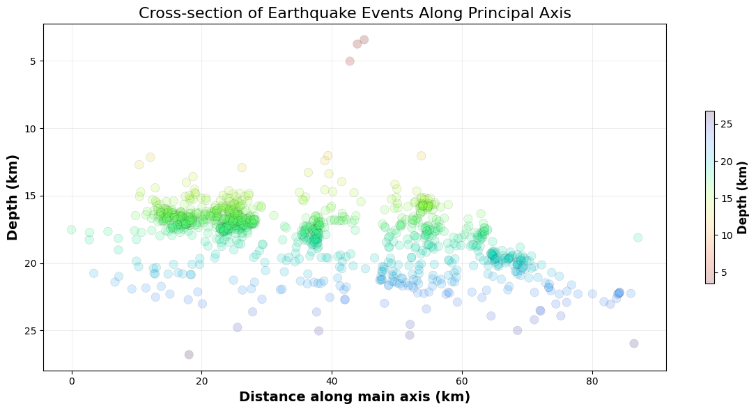
Main axis direction (LON, LAT): [0.97499714 0.2222174 ]
Explained variance ratio: 0.97
Total length of profile: 87.06 km

from sklearn.decomposition import PCA
import numpy as np

# Apply PCA to find the main axis of the earthquake cluster

# Extract coordinates for PCA
coords = events_hypodd[['LON', 'LAT']].values
pca = PCA(n_components=2)
pca.fit(coords)

# Project points onto the principal component
projected_points = pca.transform(coords)

# Convert projected points to actual distance in km using a crude approximation
# Scale factor: 1 degree ≈ 111.2 km
km_per_degree = 111.2

# Calculate the min and max in the projected space for the second component (perpendicular to main axis)
min_proj2 = projected_points[:, 1].min()
max_proj2 = projected_points[:, 1].max()

# Calculate the total span in original coordinates
second_axis_vector = pca.components_[1]  # Vector direction of second axis (LON, LAT)

# Calculate the span in degrees along the second principal axis
span_degrees2 = np.sqrt((second_axis_vector[0]**2 + second_axis_vector[1]**2)) * (max_proj2 - min_proj2)

# Convert to kilometers
span_km2 = span_degrees2 * km_per_degree

# Scale the projection to real distance in km
distance_km2 = (projected_points[:, 1] - min_proj2) * span_km2 / (max_proj2 - min_proj2)

# Create a new figure for the cross-section plot
fig, ax = plt.subplots(figsize=(12, 6))

# Plot depth vs distance across the main axis
sc = ax.scatter(distance_km2, events_hypodd['DEPTH'], 
           c=events_hypodd['DEPTH'],
           cmap='turbo_r',
           s=80,
           marker='o',
           edgecolor='k',
           linewidth=0.3,
           alpha=0.2)

# Add colorbar with shrink parameter to make it smaller
cbar = plt.colorbar(sc, ax=ax, shrink=0.5)
cbar.set_label('Depth (km)', fontsize=12, fontweight='bold')

# Set labels and title
ax.set_xlabel('Distance across fault (km)', fontsize=14, fontweight='bold')
ax.set_ylabel('Depth (km)', fontsize=14, fontweight='bold')
ax.set_title('Cross-fault Projection of Earthquake Events', fontsize=16)

# Add grid
ax.grid(True, linestyle='-', linewidth=0.5, alpha=0.4, color='gray')

# Adjust y-axis to show depth properly (negative values going down)
ax.invert_yaxis()

plt.tight_layout()
plt.show()

# Print direction of main axis for reference
main_axis_vector = pca.components_[0]
second_axis_vector = pca.components_[1]
print(f"Main axis direction (LON, LAT): {main_axis_vector}")
print(f"Second axis direction (LON, LAT): {second_axis_vector}")
print(f"Explained variance ratio: {pca.explained_variance_ratio_[0]:.2f}")
print(f"Width of cross-fault profile: {span_km2:.2f} km")

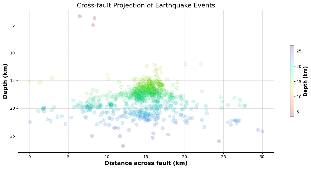
Main axis direction (LON, LAT): [0.97499714 0.2222174 ]
Second axis direction (LON, LAT): [-0.2222174   0.97499714]
Explained variance ratio: 0.97
Width of cross-fault profile: 30.03 km

Now we are going to compare before and after relocation.

# Read the original catalog for comparison
events_original = pd.read_csv('./HypoDD.loc', header=None, sep="\s+", 
                            names=['ID', 'LAT', 'LON', 'DEPTH', 'X', 'Y', 'Z', 'EX', 'EY', 'EZ', 
                                  'YR', 'MO', 'DY', 'HR', 'MI', 'SC', 'MAG', 'NCCP', 'NCCS', 'NCTP', 
                                  'NCTS', 'RCC', 'RCT', 'CID'])

# Create a figure with 2x2 grid for comparing before and after
fig = plt.figure(figsize=(15, 12))
gs = fig.add_gridspec(2, 2, width_ratios=[1.5, 1])

# Map view comparison (top-left)
ax1 = fig.add_subplot(gs[0, 0])
ax1.scatter(events_original['LON'], events_original['LAT'], c='blue', s=30, alpha=0.3, label='Original')
ax1.scatter(events_hypodd['LON'], events_hypodd['LAT'], c='red', s=30, alpha=0.3, label='HypoDD')
ax1.set_xlabel('Longitude (°)', fontsize=12)
ax1.set_ylabel('Latitude (°)', fontsize=12)
ax1.set_title('Map View: Original vs HypoDD', fontsize=14)
ax1.legend()
ax1.grid(True, linestyle='-', linewidth=0.5, alpha=0.4)
ax1.set_aspect('equal')

# Depth cross-section along longitude (top-right)
ax2 = fig.add_subplot(gs[0, 1])
ax2.scatter(events_original['LON'], events_original['DEPTH'], c='blue', s=30, alpha=0.3, label='Original')
ax2.scatter(events_hypodd['LON'], events_hypodd['DEPTH'], c='red', s=30, alpha=0.3, label='HypoDD')
ax2.set_xlabel('Longitude (°)', fontsize=12)
ax2.set_ylabel('Depth (km)', fontsize=12)
ax2.set_title('Longitude vs Depth', fontsize=14)
ax2.legend()
ax2.grid(True, linestyle='-', linewidth=0.5, alpha=0.4)
ax2.invert_yaxis()  # Depths increase downward

# Depth cross-section along latitude (bottom-left)
ax3 = fig.add_subplot(gs[1, 0])
ax3.scatter(events_original['LAT'], events_original['DEPTH'], c='blue', s=30, alpha=0.3, label='Original')
ax3.scatter(events_hypodd['LAT'], events_hypodd['DEPTH'], c='red', s=30, alpha=0.3, label='HypoDD')
ax3.set_xlabel('Latitude (°)', fontsize=12)
ax3.set_ylabel('Depth (km)', fontsize=12)
ax3.set_title('Latitude vs Depth', fontsize=14)
ax3.legend()
ax3.grid(True, linestyle='-', linewidth=0.5, alpha=0.4)
ax3.invert_yaxis()  # Depths increase downward

# Depth histogram comparison (bottom-right)
ax4 = fig.add_subplot(gs[1, 1])
ax4.hist(events_original['DEPTH'], bins=20, alpha=0.5, color='blue', label='Original')
ax4.hist(events_hypodd['DEPTH'], bins=20, alpha=0.5, color='red', label='HypoDD')
ax4.set_xlabel('Depth (km)', fontsize=12)
ax4.set_ylabel('Count', fontsize=12)
ax4.set_title('Depth Distribution', fontsize=14)
ax4.legend()
ax4.grid(True, linestyle='-', linewidth=0.5, alpha=0.4)

plt.tight_layout()
plt.show()

# Calculate and print some statistics about the differences
print(f"Mean location changes:")
print(f"  Latitude: {(events_hypodd['LAT'] - events_original['LAT']).mean():.6f} degrees")
print(f"  Longitude: {(events_hypodd['LON'] - events_original['LON']).mean():.6f} degrees")
print(f"  Depth: {(events_hypodd['DEPTH'] - events_original['DEPTH']).mean():.2f} km")
print(f"Maximum location changes:")
print(f"  Latitude: {(events_hypodd['LAT'] - events_original['LAT']).abs().max():.6f} degrees")
print(f"  Longitude: {(events_hypodd['LON'] - events_original['LON']).abs().max():.6f} degrees")
print(f"  Depth: {(events_hypodd['DEPTH'] - events_original['DEPTH']).abs().max():.2f} km")

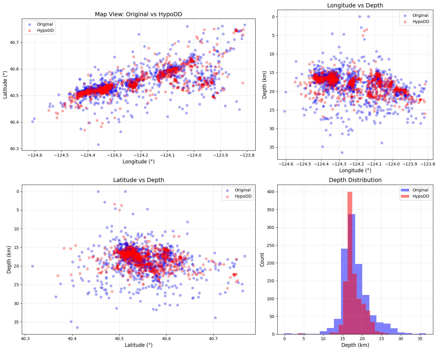
Mean location changes:
  Latitude: -0.001978 degrees
  Longitude: -0.001164 degrees
  Depth: -0.39 km
Maximum location changes:
  Latitude: 0.300660 degrees
  Longitude: 0.726135 degrees
  Depth: 19.54 km