🌐 Predicting Earthquake Origins with Graph Neural Networks#
Author: Loïc Bachelot
Goal: This notebook demonstrates how to use a GNN to predict the 2D spatial origin of synthetic seismic events from graph-structured input data.
📘 Overview#
Seismic events recorded across a geographic area generate time series data at multiple stations. To model the origin of these events:
We treat each seismic station as a node in a graph.
The edges represent relationships (e.g., geographic proximity).
The features include both the station’s location and the recorded signals.
We’ll walk through:
Creating synthetic data and graph structures
Building a GNN model (with attention-based pooling)
Training and evaluating the model
Visualizing predictions
📦 Imports and Setup#
We import PyTorch, PyTorch Geometric, and helper libraries used to build and train the GNN.
import torch
import torch_geometric
print(torch.__version__)
print(torch_geometric.__version__)
2.6.0+cu124
2.6.1
%pip install pyg_lib torch_scatter torch_sparse torch_cluster torch_spline_conv -f https://data.pyg.org/whl/torch-2.6.0+cu124.html
Looking in links: https://data.pyg.org/whl/torch-2.6.0+cu124.html
Requirement already satisfied: pyg_lib in /srv/conda/envs/notebook/lib/python3.12/site-packages (0.4.0+pt26cu124)
Requirement already satisfied: torch_scatter in /srv/conda/envs/notebook/lib/python3.12/site-packages (2.1.2+pt26cu124)
Requirement already satisfied: torch_sparse in /srv/conda/envs/notebook/lib/python3.12/site-packages (0.6.18+pt26cu124)
Requirement already satisfied: torch_cluster in /srv/conda/envs/notebook/lib/python3.12/site-packages (1.6.3+pt26cu124)
Requirement already satisfied: torch_spline_conv in /srv/conda/envs/notebook/lib/python3.12/site-packages (1.2.2+pt26cu124)
Requirement already satisfied: scipy in /srv/conda/envs/notebook/lib/python3.12/site-packages (from torch_sparse) (1.15.1)
Requirement already satisfied: numpy<2.5,>=1.23.5 in /srv/conda/envs/notebook/lib/python3.12/site-packages (from scipy->torch_sparse) (1.26.4)
Note: you may need to restart the kernel to use updated packages.
import numpy as np
import matplotlib.pyplot as plt
from torch_geometric.data import Data
import torch
import torch_geometric
from torch_geometric.transforms import KNNGraph
from torch_geometric.data import InMemoryDataset, Data
from torch.nn import Linear, Parameter, LeakyReLU, Conv2d, MaxPool1d
from torch_geometric.nn import GCNConv, MessagePassing, MLP, GATv2Conv, global_mean_pool, GlobalAttention
from scipy.spatial import distance
from torch_geometric.utils import add_self_loops, degree
from tqdm import tqdm
from torch import nn
import time
import os
print(torch.__version__)
2.6.0+cu124
🖼️ Visualization Helper Functions#
To better understand the structure of the input graphs and the behavior of the signal data, we define two visualization utilities:
visualize_graph_torch
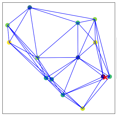
This function draws the graph in 2D space:Nodes are colored based on a given feature (e.g., signal amplitude or attention score).
Edges are shown as lines connecting nodes.
The true event origin is marked with a red ❌.
If predictions are available, the model’s estimated origin is shown with a blue ❌.
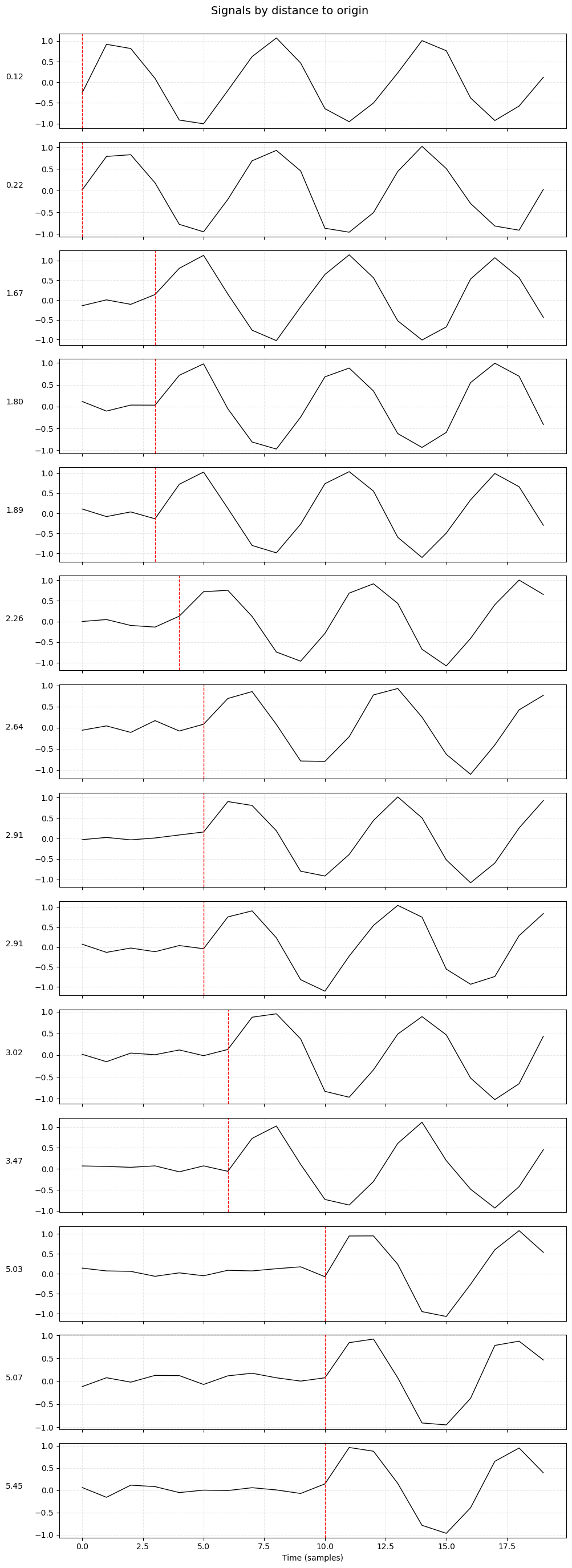
plot_signals_subplots_by_distance
This function plots the signal recorded at each station in a separate subplot:Subplots are ordered by the station’s distance from the origin.
A red dashed line indicates the expected arrival time of the wave.
This helps assess whether the signal aligns with physical expectations.
def visualize_graph_torch(g, color, pred=False, ax=None, title=None):
    """
    Visualize the graph structure with PyTorch Geometric graph object.

    Args:
        g (Data): Graph data object with edge_index, pos, and feature color
        color (str): Node attribute key to use for coloring
        pred (bool): If True, also plot predicted origin with blue cross
        ax (matplotlib.axes.Axes, optional): If provided, draw into this axis
        title (str, optional): Optional title to display above plot

    Behavior:
    - Nodes are colored by the specified feature (e.g., signal or attention score)
    - Edges are drawn in blue
    - True origin marked with red ❌
    - Prediction (if enabled) marked with blue ❌
    """
    created_fig = False
    if ax is None:
        fig, ax = plt.subplots(figsize=(6, 6))
        created_fig = True

    # Plot edges
    for edge in g.edge_index.T:
        ax.plot(
            [g.pos[edge[0]][0], g.pos[edge[1]][0]],
            [g.pos[edge[0]][1], g.pos[edge[1]][1]],
            color='blue', linewidth=1
        )

    # Node scatter with color
    scatter = ax.scatter(
        x=g.pos.T[0],
        y=g.pos.T[1],
        alpha=1,
        c=g[color][:, 0],
        s=150
    )

    # True origin
    if hasattr(g, 'y') and g.y[0].numel() == 2:
        ax.plot(g.y[0][0], g.y[0][1], 'rx', markersize=12, markeredgewidth=3)

    # Predicted origin
    if pred and hasattr(g, 'pred') and g.pred[0].numel() == 2:
        ax.plot(g.pred[0][0], g.pred[0][1], 'bx', markersize=12, markeredgewidth=3)

    # Title if given
    if title:
        ax.set_title(title)

    # Clean axes
    ax.set_xticks([])
    ax.set_yticks([])

    # Legend for coloring only once if top-level figure
    if created_fig:
        legend1 = ax.legend(*scatter.legend_elements(), loc='center left', bbox_to_anchor=(1, 0.5))
        ax.add_artist(legend1)
        plt.show()


def plot_signals_subplots_by_distance(data, velocity=0.5, sampling_rate=1.0, title="Signals by distance to origin"):
    """
    Plot each station's signal in its own subplot, ordered by distance to origin,
    with vertical lines showing the arrival time of the wavefront.

    Args:
        data (Data): PyG Data object with:
            - pos: [num_nodes, 2]
            - signal: [num_nodes, SIGNAL_SIZE]
            - y: [1, 2] or [2] for origin location
        velocity (float): Wave propagation speed (units per second)
        sampling_rate (float): Sample rate (Hz)
        title (str): Title of the figure
    """
    pos = data.pos.cpu().numpy()
    signals = data.signal.cpu().numpy()
    origin = data.y.squeeze().cpu().numpy()

    num_nodes = pos.shape[0]

    # Compute distances from origin and convert to sample index
    distances = np.array([distance.euclidean(origin, pos[i].tolist()) for i in range(num_nodes)])
    arrival_samples = (distances / velocity * sampling_rate).astype(int)
    sort_idx = np.argsort(distances)

    # Plot one subplot per station
    fig, axs = plt.subplots(num_nodes, 1, figsize=(10, 2 * num_nodes), sharex=True)
    for i, idx in enumerate(sort_idx):
        ax = axs[i]
        signal = signals[idx]

        ax.plot(np.arange(len(signal)), signal, color='black', linewidth=1)
        ax.axvline(arrival_samples[idx], color='red', linestyle='--', linewidth=1, label='arrival')
        ax.set_ylabel(f"{distances[idx]:.2f}", rotation=0, labelpad=25)
        ax.grid(True, linestyle='--', alpha=0.3)

    axs[-1].set_xlabel("Time (samples)")
    fig.suptitle(title, fontsize=14)
    plt.tight_layout(rect=[0, 0, 1, 0.98])
    plt.show()
📈 Synthetic Dataset Creation#
We simulate synthetic graph-based seismic data to train our Graph Neural Network (GNN). Each graph represents a seismic network where:
Nodes are seismic stations with 2D spatial coordinates.
Edges are created later based on k-nearest neighbors or distance.
Signals at each station are generated as noisy sine waves, delayed in time based on the distance to a hidden origin (the earthquake location).
The target (
y) for each graph is the 2D coordinate of the origin — the same for all nodes.
🧪 Signal Generation Parameters:#
nb_nodes ∈ [10, 15]: Number of seismic stations per graph.origin ∈ [0, 6]²: The true epicenter is sampled randomly in a 6×6 unit grid.velocity = 0.5 units/sec: Controls how fast the signal propagates from the origin.sampling_rate = 1.0 Hz: Defines the number of samples per unit of time.noise_std = 0.1: Gaussian noise is added to simulate real-world signal variation.SIGNAL_SIZE: Total number of samples in the signal window (e.g., 100).
🌀 How are signals delayed?#
The signal at each node starts with random noise. Then:
The time delay is computed as
distance / velocityConverted to a sample index:
delay_samples = delay * sampling_rateA sine wave is inserted at this delayed position in the signal
This creates a physically intuitive training signal: stations farther from the source receive the waveform later in time.
This setup allows the GNN to learn to infer the origin coordinates purely from the spatial pattern of waveform arrivals and features across nodes.
def add_edge_weight(g):
    """
    Compute edge weights based on inverse distance between nodes.

    This function adds an 'edge_weight' attribute to each graph,
    calculated as 1 / (distance + 1) to ensure numerical stability.

    Args:
        g (Data): PyG graph with 'pos' and 'edge_index'

    Returns:
        Data: Modified graph with 'edge_weight'
    """
    edge_weight = []
    for edge in g.edge_index.T:
        node_a, node_b = g.pos[edge[0]], g.pos[edge[1]]
        dist = distance.euclidean((node_a[0], node_a[1]), (node_b[0], node_b[1]))
        edge_weight.append(1 / (dist + 1))  # add 1 to avoid division by zero
    g.edge_weight = torch.tensor(np.array(edge_weight)).type(torch.FloatTensor)
    return g


class SinOriginDataset(InMemoryDataset):
    """
    Synthetic dataset for training GNNs to predict origin locations.

    Each graph in the dataset includes:
    - Randomly placed nodes in 2D space.
    - Sine wave signals at each node, delayed by distance from a hidden origin.
    - A regression target: the origin coordinates.

    Args:
        root (str): Root directory to save the processed data
        nb_graph (int): Number of synthetic graphs to generate
    """
    def __init__(self, root, transform=None, pre_transform=None, nb_graph=10):
        self.nb_graph = nb_graph
        super(SinOriginDataset, self).__init__(root, transform, pre_transform)
        self.data, self.slices = torch.load(self.processed_paths[0], weights_only=False)

    @property
    def raw_file_names(self):
        # No raw input files; data is generated from scratch
        return 0

    @property
    def processed_file_names(self):
        return 'data.pt'

    def process(self):
        data_list = []

        # Dataset parameters
        frequency = 1.0        # Hz
        velocity = 0.5         # wave speed
        sampling_rate = 1.0    # Hz
        noise_std = 0.1        # Gaussian noise level

        # Base sine wave used in signal synthesis
        base_sine_wave = np.sin(np.arange(SIGNAL_SIZE))

        for _ in range(self.nb_graph):
            nb_nodes = np.random.randint(10, 15)  # Graph size
            pos = torch.tensor(np.random.uniform(0, 6, size=(nb_nodes, 2)), dtype=torch.float)  # Node positions
            origin = np.random.randint(0, 6, size=2)  # True origin
            origin_tensor = torch.tensor(origin, dtype=torch.float)

            signal_list = []
            for i in range(nb_nodes):
                dist = distance.euclidean(origin, pos[i].tolist())
                delay = dist / velocity
                delay_samples = int(delay * sampling_rate)

                # Start with noise
                waveform = np.random.normal(0, noise_std, size=SIGNAL_SIZE)

                # Add delayed sine wave if within bounds
                if delay_samples < SIGNAL_SIZE:
                    insert_length = SIGNAL_SIZE - delay_samples
                    waveform[delay_samples:] += base_sine_wave[:insert_length]

                signal_list.append(waveform)

            signal = torch.tensor(np.array(signal_list), dtype=torch.float32).reshape(nb_nodes, SIGNAL_SIZE)
            g = Data(pos=pos, signal=signal, y=origin_tensor.unsqueeze(0))  # y shape: (1, 2)
            data_list.append(g)

        # Apply graph transformations if provided (e.g., KNN, edge weights)
        if self.pre_transform is not None:
            data_list = [self.pre_transform(data) for data in data_list]
            data_list = [add_edge_weight(data) for data in data_list]

        # Save to disk
        data, slices = self.collate(data_list)
        torch.save((data, slices), self.processed_paths[0])
SIGNAL_SIZE = 20
NB_GRAPHS = 1000

raw_dataset = SinOriginDataset(root="./sin_train", pre_transform=KNNGraph(k=5, loop=False, force_undirected=True),
                       nb_graph=NB_GRAPHS)
raw_dataset
SinOriginDataset(1000)
🔍 Exploring a Graph Sample#
Let’s take a look at one sample from our synthetic dataset to understand its structure.
PyTorch Geometric stores each graph in a Data object. Here’s what each attribute means:
y=[1, 2]: The target — the 2D coordinates of the true origin (shared by all nodes in the graph).pos=[13, 2]: The 2D spatial positions of 13 nodes (i.e., seismic stations).signal=[13, 20]: Each node has a 1D signal of length 20 (e.g., amplitude over time).edge_index=[2, 74]: The graph has 74 directed edges represented as source/target pairs.edge_weight=[74]: Weights for each edge, inversely proportional to spatial distance.
This compact format allows the GNN to process signals in a way that respects the spatial relationships between nodes.
data = raw_dataset[0]
data
Data(y=[1, 2], pos=[14, 2], signal=[14, 20], edge_index=[2, 84], edge_weight=[84])
visualize_graph_torch(data, color='signal')
plot_signals_subplots_by_distance(data)
🔄 Target Normalization#
Before training the model, we normalize the target coordinates (i.e., the true origin) to fall within a standard range.
This is a common preprocessing step in regression problems, especially when using neural networks, because:
It helps with training stability and convergence.
Activations remain within consistent ranges.
The network doesn’t need to “learn” scale information from scratch.
We define a wrapper class NormalizeTargetsWrapper that rescales the target y values from their original coordinate bounds (e.g., [0, 6]) to the range [-1, 1]. This normalized range works well with activation functions like tanh.
The class also includes a denormalize() method, which maps predictions back to the original coordinate space for evaluation and visualization.
class NormalizeTargetsWrapper(torch.utils.data.Dataset):
    """
    Wraps a PyG dataset to normalize `y` from [min_val, max_val] → [-1, 1].
    """
    def __init__(self, dataset, min_val, max_val):
        self.dataset = dataset
        self.min_val = min_val
        self.max_val = max_val

    def __len__(self):
        return len(self.dataset)

    def __getitem__(self, idx):
        data = self.dataset[idx].clone()
        # scale from [min, max] to [-1, 1]
        data.y = 2 * (data.y - self.min_val) / (self.max_val - self.min_val) - 1
        return data

    def denormalize(self, norm_y):
        # scale back from [-1, 1] to [min, max]
        return 0.5 * (norm_y + 1) * (self.max_val - self.min_val) + self.min_val
normalized_dataset = NormalizeTargetsWrapper(raw_dataset, min_val=0, max_val=6)
Train/Validation/Test Split and Batching#
We split the dataset into three parts:
50% for training
40% of the remaining for validation
10% for testing
Using torch_geometric.loader.DataLoader, we then batch graphs together for efficient training.
🧱 How batching works in PyTorch Geometric:#
Unlike image datasets, where each batch is a simple tensor stack, in PyG, batching involves:
Merging node and edge attributes from multiple graphs
Tracking which nodes belong to which graph using a
batchvectorAllowing global pooling operations like
GlobalAttentionto work on per-graph basis
Each batch now behaves like a single big disconnected graph, where GNN layers operate seamlessly across all examples.
We set batch_size=64 for all splits and enable shuffling only for training.
from torch_geometric.loader import DataLoader
from sklearn.model_selection import train_test_split

train_dataset, val_dataset = train_test_split(normalized_dataset, train_size=0.5, random_state=42)
val_dataset, test_dataset = train_test_split(val_dataset, train_size=0.8, random_state=42)

train_loader = DataLoader(train_dataset, batch_size=64, shuffle=True)
val_loader = DataLoader(val_dataset, batch_size=64, shuffle=False)
test_loader = DataLoader(test_dataset, batch_size=64, shuffle=False)


print(f"nb graph train ds= {len(train_dataset)}, nb graph val ds= {len(val_dataset)}, nb graph test ds= {len(test_dataset)}")
nb graph train ds= 500, nb graph val ds= 400, nb graph test ds= 100
🧠 GNN Model Definition: MLPNet#
We now define our graph neural network model, MLPNet, which predicts the origin coordinates of a seismic event from the structure and signals of a graph.
🏗️ Architecture Overview:#
Input Features:
We concatenate each node’s 2D position with its signal vector.MLP Encoder (
mlp_in):
A multi-layer perceptron (MLP) maps the concatenated input to a hidden representation.Graph Attention Layers (
conv1,conv2):
TwoGATv2Convlayers apply self-attention across neighboring nodes, using edge weights (inversely proportional to distance).🔁 Note: Only
conv1is used here;conv2is commented out, for model simplification, but showing the possibility to extend the number of message passing layers.MLP Decoder (
mlp_out):
Another MLP refines node embeddings after message passing.Global Attention Pooling (
att_pool):
Aggregates node features into a single graph-level vector using learnable attention weights (viaGlobalAttention).Final Linear Output (
out_linear):
Predicts a 2D coordinate from the pooled graph representation, constrained to [-1, 1] viatanh().
📤 Output:#
A single 2D coordinate per graph, representing the model’s normalized prediction of the origin.
This architecture combines local (node-level) feature transformations with global (graph-level) aggregation, making it well-suited for spatial inference tasks like epicenter localization.
class MLPNet(torch.nn.Module):
    """
    GNN model with MLP → 2x GATv2Conv → MLP for graph-level origin prediction.

    Args:
        channels_x (int): Positional input features per node.
        channels_y (int): Signal features per node.
        hidden_channels (int): Hidden dimension.
        dropout (float): Dropout probability.
        self_loops (bool): Whether to add self-loops to GATv2Conv.

    Output:
        Tensor of shape (batch_size, 2), normalized origin coordinates (in [-1, 1]).
    """
    def __init__(self, channels_x, channels_y, hidden_channels=128, dropout=0.3, self_loops=True):
        super(MLPNet, self).__init__()
        torch.manual_seed(1234)

        self.mlp_in = MLP([channels_x + channels_y, 64, hidden_channels])

        self.conv1 = GATv2Conv(
            in_channels=hidden_channels,
            out_channels=hidden_channels,
            heads=2,
            edge_dim=1,
            add_self_loops=self_loops,
            concat=True
        )

        self.conv2 = GATv2Conv(
            in_channels=hidden_channels * 2,  # output of conv1 with 2 heads
            out_channels=hidden_channels,
            heads=2,
            edge_dim=1,
            add_self_loops=self_loops,
            concat=True
        )

        self.mlp_out = MLP([hidden_channels * 2, 64], act=nn.LeakyReLU(), dropout=dropout)

        self.att_pool = GlobalAttention(
            gate_nn=torch.nn.Sequential(
                nn.Linear(64, 32),
                nn.ReLU(),
                nn.Linear(32, 1)
            )
        )

        self.out_linear = Linear(64, 2)

    def forward(self, pos, signal, edge_index, edge_weight, batch=None):
        x = torch.cat([pos, signal], dim=-1)
        x = self.mlp_in(x)
        x = self.conv1(x, edge_index, edge_weight)
        # x = self.conv2(x, edge_index, edge_weight)
        x = self.mlp_out(x)

        if batch is None:
            batch = torch.zeros(x.size(0), dtype=torch.long, device=x.device)

        graph_repr = self.att_pool(x, batch)
        return self.out_linear(graph_repr).tanh()
🚀 Training Loop#
This section defines the training and validation routines for our GNN model, as well as a simple early stopping mechanism.
🛠️ Helper Functions#
Before starting the main loop, we define:
EarlyStopper
A utility class to stop training when the validation loss plateaus. It tracks the lowest validation loss seen and stops training if no improvement is observed for a specified number of epochs (patience).train()
Runs one full training epoch:Iterates over batched graphs
Computes predictions and loss
Updates model weights using backpropagation
validation()
Evaluates the model on a validation set without updating weights. This is used to monitor overfitting and trigger early stopping.
ℹ️ Both
train()andvalidation()rely on:
The global
model,optimizer, andcriterionBatched data from
torch_geometric.loader.DataLoader.to(device)to move data to the appropriate compute device (e.g., GPU)
class EarlyStopper:
    """
    A class for early stopping the training process when the validation loss stops improving.
    """
    def __init__(self, patience=1, min_delta=0):
        self.patience = patience
        self.min_delta = min_delta
        self.counter = 0
        self.min_validation_loss = np.inf

    def early_stop(self, validation_loss):
        if validation_loss < self.min_validation_loss:
            self.min_validation_loss = validation_loss
            self.counter = 0
        elif validation_loss > (self.min_validation_loss + self.min_delta):
            self.counter += 1
            if self.counter >= self.patience:
                return True
        return False


def train(dataloader, device):
    model.train()
    mean_loss = 0
    for data in dataloader:
        data = data.to(device)
        optimizer.zero_grad()

        # Forward pass
        pred = model(data.pos, data.signal, data.edge_index, data.edge_weight, data.batch)  # → shape [num_graphs, 2]

        # Check shape of target
        assert data.y.shape == pred.shape, f"Expected y shape {pred.shape}, got {data.y.shape}"

        loss = criterion(pred, data.y)
        loss.backward()
        optimizer.step()
        mean_loss += loss.item()
    return mean_loss / len(dataloader)


@torch.no_grad()
def validation(dataloader, device):
    model.eval()
    total_loss = 0
    for data in dataloader:
        data = data.to(device)
        pred = model(data.pos, data.signal, data.edge_index, data.edge_weight, data.batch)
        loss = criterion(pred, data.y)
        total_loss += loss.item()
    return total_loss / len(dataloader)
⚙️ Training Setup#
Before launching training:
We select a compute device (GPU if available).
Instantiate the
MLPNetmodel.Use Mean Squared Error (MSE) as the loss function — ideal for continuous coordinate regression.
Choose the Adam optimizer with a learning rate of
1e-4.Initialize the
EarlyStopperto monitor validation loss and prevent overfitting.Set up a checkpointing path to save the best model based on validation performance.
device = torch.device('cuda:0' if torch.cuda.is_available() else 'cpu')

model = MLPNet(data.pos.shape[1], data.signal.shape[1], hidden_channels=64)

criterion = torch.nn.MSELoss()  # Define loss criterion.
optimizer = torch.optim.Adam(model.parameters(), lr=0.0001)  # Define optimizer.
early_stopper = EarlyStopper(patience=1, min_delta=0.0)
loss_train = []
loss_val = []
best_loss = 1
best_epoch = 0
PATH_CHECKPOINT = "./checkpoint/best_origin_pred.pt"
# Create the folder if it doesn't exist
os.makedirs(os.path.dirname(PATH_CHECKPOINT), exist_ok=True)
model
/srv/conda/envs/notebook/lib/python3.12/site-packages/torch_geometric/deprecation.py:26: UserWarning: 'nn.glob.GlobalAttention' is deprecated, use 'nn.aggr.AttentionalAggregation' instead
  warnings.warn(out)
MLPNet(
  (mlp_in): MLP(22, 64, 64)
  (conv1): GATv2Conv(64, 64, heads=2)
  (conv2): GATv2Conv(128, 64, heads=2)
  (mlp_out): MLP(128, 64)
  (att_pool): GlobalAttention(gate_nn=Sequential(
    (0): Linear(in_features=64, out_features=32, bias=True)
    (1): ReLU()
    (2): Linear(in_features=32, out_features=1, bias=True)
  ), nn=None)
  (out_linear): Linear(in_features=64, out_features=2, bias=True)
)
🔁 Training Loop#
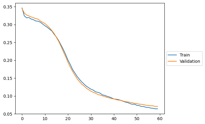
The loop runs for up to 5000 epochs, or until early stopping is triggered. At each epoch:
We compute and store the training and validation losses.
Save the model whenever a new best validation loss is observed.
Use
tqdmto display a real-time progress bar with current losses.
🧠 Note: Early stopping helps avoid unnecessary training once the model stops improving.
start_time = time.perf_counter()
nb_epoch = tqdm(range(5000))

for epoch in nb_epoch:
    loss_train.append(train(train_loader, device))
    loss_val.append(validation(val_loader, device))

    if loss_val[-1] < best_loss:
        best_loss = loss_val[-1]
        best_epoch = epoch
        torch.save(model.state_dict(), PATH_CHECKPOINT)
    if early_stopper.early_stop(loss_val[-1]):
        print(f"early stopping at epoch {epoch}: train loss={loss_train[-1]}, val loss={loss_val[-1]}")
        break
    nb_epoch.set_postfix_str(f"train loss={loss_train[-1]}, val loss={loss_val[-1]}")
1%| | 59/5000 [00:12<17:40, 4.66it/s, train loss=0.06399355875328183, val loss=0.07068957335182599]
early stopping at epoch 59: train loss=0.0641244943253696, val loss=0.07113602384924889
plt.plot(loss_train, label="Train")
plt.plot(loss_val, label = "Validation")
plt.legend(loc='center left', bbox_to_anchor=(1, 0.5))
<matplotlib.legend.Legend at 0x7f1843f08830>
📈 Model Evaluation#
After training, we assess how well the model generalizes to unseen data.
The evaluation process includes:
Load Best Model Checkpoint
We reload the model weights corresponding to the best validation loss during training. This ensures that we evaluate the most performant version of the model, not just the final state.Visual Inspection on a Few Graphs
We make predictions on a small set of random graphs from the test set.Visualize predicted vs true origin positions.
Get an intuitive feel for typical prediction quality.
Full Test Set Prediction
We then predict on the entire test set to quantify performance over a larger sample.Compute Simple Metrics
We calculate basic metrics such as:Mean Absolute Error (MAE) between predicted and true coordinates
Optionally visualize prediction error distributions
🧠 This evaluation allows both qualitative (plots) and quantitative (error metrics) understanding of model performance.
# restore best model
# PATH_CHECKPOINT = "./checkpoint/best_origin_pred.pt"
model.load_state_dict(torch.load(PATH_CHECKPOINT))
print(f"best loss={best_loss}, model eval loss={validation(test_dataset, device)} at epoch {best_epoch}")
best loss=0.07068957335182599, model eval loss=0.05902902354137041 at epoch 58
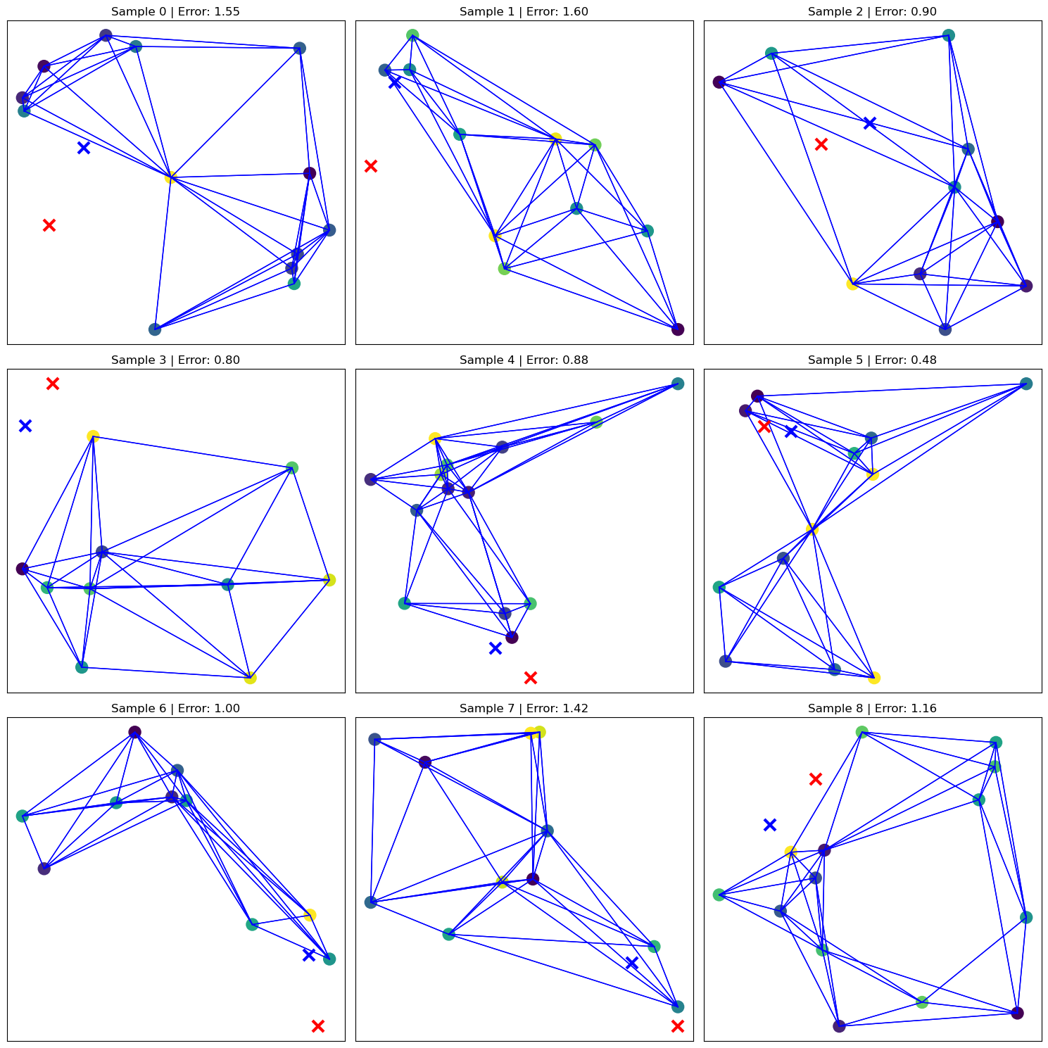
🔍 Visualizing Predictions on 9 Test Graphs#
To qualitatively evaluate the model’s spatial accuracy, we display predictions on 9 test graphs using a 3×3 grid.
Each subplot shows:
The graph structure and node positions
Node coloring based on signal values
The true origin (red ❌) and predicted origin (blue ❌)
The per-sample Euclidean error in the title
This visualization helps identify both successful and challenging prediction scenarios.
fig, axs = plt.subplots(3, 3, figsize=(15, 15))
axs = axs.flatten()

for i in range(9):
    data = test_dataset[i].clone().to(device)

    with torch.no_grad():
        pred = model(data.pos, data.signal, data.edge_index, data.edge_weight, batch=None)

    data.pred = normalized_dataset.denormalize(pred)
    data.y = normalized_dataset.denormalize(data.y)
    data.error = torch.norm(data.pred - data.y, dim=-1).unsqueeze(0)

    ax = axs[i]
    # Custom version of visualize_graph_torch that plots into a given `ax`
    visualize_graph_torch(data, color="signal", pred=True, ax=ax)
    ax.set_title(f"Sample {i} | Error: {data.error.item():.2f}")

plt.tight_layout()
plt.show()
📊 Quantitative Evaluation and Error Distribution#
We compute a set of quantitative metrics over the full test set to assess the model’s predictive accuracy.
🧮 Reported Metrics:#
MAE (Mean Absolute Error) for X and Y separately
Total MAE across both dimensions
RMSE (Root Mean Squared Error) — penalizes larger errors more heavily
Mean Euclidean Error — distance between predicted and true origin
Max Euclidean Error — worst-case prediction
These metrics provide a robust summary of how well the model generalizes.
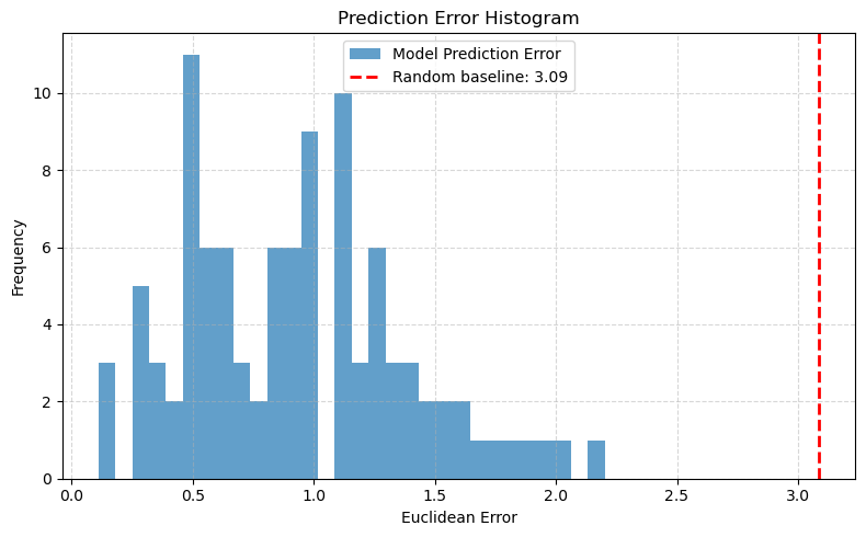
📉 Error Histogram:#
We also visualize the distribution of Euclidean errors across all test samples.
A red dashed line shows the expected error from a random guess, providing a baseline reference.
The histogram reveals whether the model consistently predicts near the true origin — or struggles in specific regions.
@torch.no_grad()
def evaluate(model, test_loader, normalized_dataset, device):
    """
    Evaluate model on the full test set and compute error metrics.

    Returns:
        Dict of evaluation metrics
    """
    model.eval()

    pred_all = []
    true_all = []

    for data in test_loader:
        data = data.to(device)
        pred = model(data.pos, data.signal, data.edge_index, data.edge_weight, data.batch)

        pred_denorm = normalized_dataset.denormalize(pred)
        true_denorm = normalized_dataset.denormalize(data.y)

        pred_all.append(pred_denorm.cpu())
        true_all.append(true_denorm.cpu())

    pred_all = torch.cat(pred_all, dim=0)
    true_all = torch.cat(true_all, dim=0)

    abs_errors = torch.abs(pred_all - true_all)
    euclidean_errors = torch.norm(pred_all - true_all, dim=1)

    metrics = {
        "MAE_x": abs_errors[:, 0].mean().item(),
        "MAE_y": abs_errors[:, 1].mean().item(),
        "MAE_total": abs_errors.mean().item(),
        "RMSE": torch.sqrt(((pred_all - true_all) ** 2).mean()).item(),
        "Mean Euclidean Error": euclidean_errors.mean().item(),
        "Max Euclidean Error": euclidean_errors.max().item()
    }

    for k, v in metrics.items():
        print(f"{k}: {v:.3f}")

    return metrics, pred_all, true_all

def plot_error_histogram(pred_all, true_all, bounds=(0, 6), bins=30):
    """
    Plot a histogram of Euclidean errors with optional random baseline.

    Args:
        pred_all (Tensor): shape [N, 2], model predictions (denormalized)
        true_all (Tensor): shape [N, 2], true targets (denormalized)
        bounds (tuple): min/max coordinate bounds for random baseline
        bins (int): histogram bin count
    """
    # Compute Euclidean errors
    errors = torch.norm(pred_all - true_all, dim=1).numpy()

    # Estimate expected error from random predictions in the same domain
    num_samples = len(pred_all)
    rand_preds = torch.rand_like(pred_all) * (bounds[1] - bounds[0]) + bounds[0]
    rand_errors = torch.norm(rand_preds - true_all, dim=1).numpy()
    expected_random_error = rand_errors.mean()

    # Plot
    plt.figure(figsize=(8, 5))
    plt.hist(errors, bins=bins, alpha=0.7, label="Model Prediction Error")
    plt.axvline(expected_random_error, color="red", linestyle="--", linewidth=2,
                label=f"Random baseline: {expected_random_error:.2f}")
    plt.xlabel("Euclidean Error")
    plt.ylabel("Frequency")
    plt.title("Prediction Error Histogram")
    plt.legend()
    plt.grid(True, linestyle="--", alpha=0.5)
    plt.tight_layout()
    plt.show()
metrics, pred_all, true_all = evaluate(model, test_loader, normalized_dataset, device)

# reuse prediction and truth tensors
plot_error_histogram(pred_all, true_all, bounds=(0, 6))
MAE_x: 0.562
MAE_y: 0.614
MAE_total: 0.588
RMSE: 0.729
Mean Euclidean Error: 0.926
Max Euclidean Error: 2.202
✅ Conclusion#
In this notebook, we built and evaluated a Graph Neural Network (GNN) to predict 2D origin coordinates from synthetic seismic-like signals distributed across a spatial graph.
🧠 What We Did:#
Generated a toy dataset of sine signals delayed by distance to a hidden origin.
Encoded both spatial (
pos) and signal features for each node.Used GATv2Conv layers and Global Attention Pooling to learn graph-level representations.
Normalized targets for stable training and evaluated with metrics like MAE and RMSE.
Visualized predictions at both the graph-level and dataset-level.
📊 What We Learned:#
GNNs can effectively model spatial dependencies and delays in signal propagation.
Attention-based pooling enables flexible aggregation of node-level features.
Even in a simplified setting, errors remain spatially structured — indicating areas where the model struggles (e.g., sparse graphs or boundary cases).
🧭 Next Steps:#
Try more complex synthetic scenarios: include signal polarity, noise bursts, or multi-event graphs.
Use real waveform datasets (e.g., from SeisBench) with station metadata.
Experiment with alternate architectures: GINConv, Transformer-based pooling, or EdgeConv.
Add uncertainty estimation or confidence bounds to predictions.
🚀 GNNs are powerful tools for modeling geospatial and physical systems — and this notebook is just a start!