British Columbia Landslide Data Preprocessing#
Overview#
This notebook processes landslide data from British Columbia for integration with the Cascadia regional dataset.
Key Processing Steps:#
Load National Dataset: Import Canadian landslide database from CSV (https://data.niaid.nih.gov/resources?id=zenodo_7089351)
Geographic Filtering: Extract British Columbia records using coordinate boundaries
Standardization: Align column names and data types with unified schema
Export Processing: Save cleaned data as standardized GeoJSON
Initial Inspection#
import geopandas as gpd
import pandas as pd
import matplotlib.pyplot as plt
import seaborn as sns
gdf = gpd.read_file("../data/Canada/Canadian_landslide_database_February2025_version10.1.csv")
len(gdf)
11135
gdf.head()
| LS_ID | Name | Longitude | Latitude | Type | Material | Size_class | Timing | Trigger | Contributo | ... | Study_area | Watercours | Event_verification | Volume_estimate_method | Discharge estimate (m3/s) | Deposit_Arrea_m2 | Bedrock_type | Point_location | Location_confidence | Comment | |
|---|---|---|---|---|---|---|---|---|---|---|---|---|---|---|---|---|---|---|---|---|---|
| 0 | LS00001 | Clinton Creek Mine | -140.7341 | 64.446393000000000 | Debris avalanche | Anthropogenic | 1974 | ... | 0 | 0 | Headscarp | High | Landslide dammed lake | ||||||||
| 1 | LS00002 | Old alignment failure | -140.1726 | 64.224711769999999 | Debris avalanche | Surficial | ... | 0 | 0 | Headscarp | High | ||||||||||
| 2 | LS00003 | Horseshoe Bay debris avalanche | -138.5108 | 61.040703000000001 | Debris avalanche | Surficial | ... | 0 | 0 | Headscarp | High | ||||||||||
| 3 | LS00004 | Small debris avalanche | -138.0579 | 61.448892479999998 | Debris avalanche | Surficial | ... | 0 | 0 | Headscarp | High | ||||||||||
| 4 | LS00005 | Volcano Mountain | -137.3798 | 62.921592720000000 | Debris avalanche | Surficial | ... | 0 | 0 | Headscarp | Moderate |
5 rows × 25 columns
Filter out British Columbia#
# Filter for British Columbia based on longitude and latitude
# -130, 52 and -116, 52
bc_gdf = gdf[(gdf['Longitude'].astype(float) >= -130) &
             (gdf['Longitude'].astype(float) <= -116) &
             (gdf['Latitude'].astype(float) <= 52) ]

print(f"Number of records in BC: {len(bc_gdf)}")
bc_gdf.head()
Number of records in BC: 4461
| LS_ID | Name | Longitude | Latitude | Type | Material | Size_class | Timing | Trigger | Contributo | ... | Study_area | Watercours | Event_verification | Volume_estimate_method | Discharge estimate (m3/s) | Deposit_Arrea_m2 | Bedrock_type | Point_location | Location_confidence | Comment | |
|---|---|---|---|---|---|---|---|---|---|---|---|---|---|---|---|---|---|---|---|---|---|
| 86 | LS00087 | Debris avalanche | -128.1971 | 50.533960000000000 | Debris avalanche | Surficial | ... | 0 | 0 | Headscarp | High | ||||||||||
| 87 | LS00088 | Debris avalanche | -128.187 | 50.535750000000000 | Debris avalanche | Surficial | ... | 0 | 0 | Headscarp | High | ||||||||||
| 88 | LS00089 | Debris avalanche | -128.1838 | 50.530299999999997 | Debris avalanche | Surficial | ... | 0 | 0 | Headscarp | High | ||||||||||
| 89 | LS00090 | Debris avalanche | -128.1819 | 50.531920000000000 | Debris avalanche | Surficial | ... | 0 | 0 | Headscarp | High | ||||||||||
| 90 | LS00091 | Debris avalanche | -128.1769 | 50.540880000000001 | Debris avalanche | Surficial | ... | 0 | 0 | Headscarp | High |
5 rows × 25 columns
# Convert Longitude and Latitude to numeric types, coercing errors to NaN
bc_gdf['Longitude'] = pd.to_numeric(bc_gdf['Longitude'], errors='coerce')
bc_gdf['Latitude'] = pd.to_numeric(bc_gdf['Latitude'], errors='coerce')
# Drop rows with invalid coordinate values
bc_gdf.dropna(subset=['Longitude', 'Latitude'], inplace=True)
# Create a GeoDataFrame with point geometries
bc_gdf = gpd.GeoDataFrame(
bc_gdf, geometry=gpd.points_from_xy(bc_gdf.Longitude, bc_gdf.Latitude))
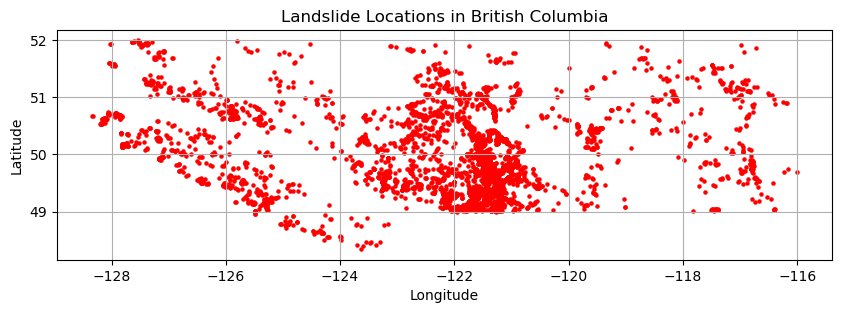
# Plot the data
fig, ax = plt.subplots(1, 1, figsize=(10, 10))
bc_gdf.plot(ax=ax, marker='o', color='red', markersize=5)
plt.title("Landslide Locations in British Columbia")
plt.xlabel("Longitude")
plt.ylabel("Latitude")
plt.grid(True)
plt.show()
C:\Users\loicb\AppData\Local\Temp\ipykernel_25496\2027393985.py:2: SettingWithCopyWarning:
A value is trying to be set on a copy of a slice from a DataFrame.
Try using .loc[row_indexer,col_indexer] = value instead

See the caveats in the documentation: https://pandas.pydata.org/pandas-docs/stable/user_guide/indexing.html#returning-a-view-versus-a-copy
  bc_gdf['Longitude'] = pd.to_numeric(bc_gdf['Longitude'], errors='coerce')
C:\Users\loicb\AppData\Local\Temp\ipykernel_25496\2027393985.py:3: SettingWithCopyWarning:
A value is trying to be set on a copy of a slice from a DataFrame.
Try using .loc[row_indexer,col_indexer] = value instead

See the caveats in the documentation: https://pandas.pydata.org/pandas-docs/stable/user_guide/indexing.html#returning-a-view-versus-a-copy
  bc_gdf['Latitude'] = pd.to_numeric(bc_gdf['Latitude'], errors='coerce')
C:\Users\loicb\AppData\Local\Temp\ipykernel_25496\2027393985.py:6: SettingWithCopyWarning:
A value is trying to be set on a copy of a slice from a DataFrame

See the caveats in the documentation: https://pandas.pydata.org/pandas-docs/stable/user_guide/indexing.html#returning-a-view-versus-a-copy
  bc_gdf.dropna(subset=['Longitude', 'Latitude'], inplace=True)
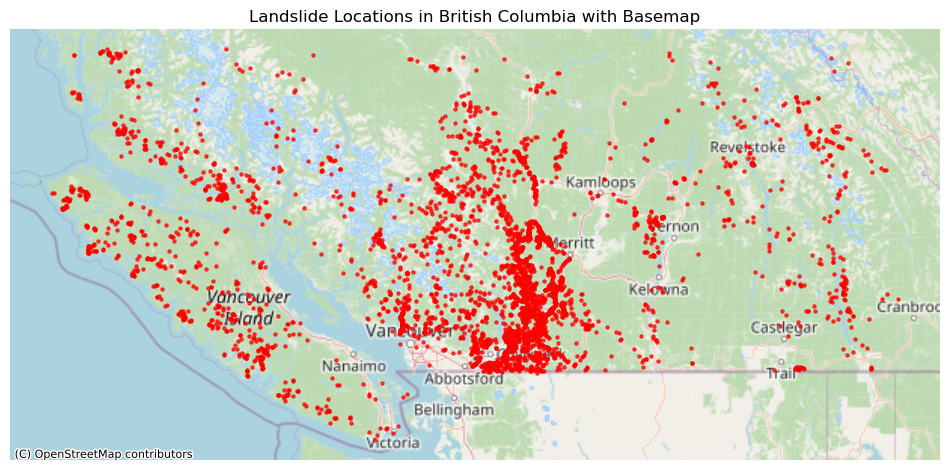
import contextily as ctx

if bc_gdf.crs is None:
    bc_gdf.set_crs(epsg=4326, inplace=True)

# Create the plot
fig, ax = plt.subplots(1, 1, figsize=(12, 12))

# Plot the landslide data
bc_gdf.to_crs(epsg=3857).plot(ax=ax, marker='o', color='red', markersize=5, alpha=0.7, label='Landslides')

# Add the basemap
ctx.add_basemap(ax, source=ctx.providers.OpenStreetMap.Mapnik)

# Customize the plot
ax.set_title("Landslide Locations in British Columbia with Basemap")
ax.set_axis_off() # The basemap provides the geographic context
plt.show()
Analysis#
# Seperating deposits by column types
numerical_cols = gdf.select_dtypes(include=['number']).columns.tolist()

non_numerical_cols = gdf.select_dtypes(exclude=['number']).columns.tolist()
print("Numerical Columns:")
for col in numerical_cols:
    print(f"  - {col}")

print("\nNon-Numerical Columns:")
for col in non_numerical_cols:
    print(f"  - {col}")
Numerical Columns:

Non-Numerical Columns:
  - LS_ID
  - Name
  - Longitude
  - Latitude
  - Type
  - Material
  - Size_class
  - Timing
  - Trigger
  - Contributo
  - Reference
  - Type_details
  - Cont_details
  - Resource_road_activity
  - Resource_road_type
  - Study_area
  - Watercours
  - Event_verification
  - Volume_estimate_method
  - Discharge estimate (m3/s)
  - Deposit_Arrea_m2
  - Bedrock_type
  - Point_location
  - Location_confidence
  - Comment
New Columns#
Confidence#
We will convert the values into 3 main classes Moderate, High and Low to be more consistent with Washington and Oregon.
Raw Confidence Values#
print("Value Counts for Location Confidence:")
print(bc_gdf['Location_confidence'].value_counts())
Value Counts for Location Confidence:
Location_confidence
High        3320
             947
Moderate     176
Low           18
Name: count, dtype: int64
Replacing empty strings with NaN#
import numpy as np

# Replace empty strings with NaN
bc_gdf['Location_confidence'].replace('', np.nan, inplace=True)

print("Updated Value Counts for Location Confidence:")
print(bc_gdf['Location_confidence'].value_counts())
Updated Value Counts for Location Confidence:
Location_confidence
High        3320
Moderate     176
Low           18
Name: count, dtype: int64
C:\Users\loicb\AppData\Local\Temp\ipykernel_25496\35487707.py:4: FutureWarning: A value is trying to be set on a copy of a DataFrame or Series through chained assignment using an inplace method.
The behavior will change in pandas 3.0. This inplace method will never work because the intermediate object on which we are setting values always behaves as a copy.

For example, when doing 'df[col].method(value, inplace=True)', try using 'df.method({col: value}, inplace=True)' or df[col] = df[col].method(value) instead, to perform the operation inplace on the original object.


  bc_gdf['Location_confidence'].replace('', np.nan, inplace=True)
Type#
Original Type#
type_counts = bc_gdf['Type'].value_counts()
print("\nValue Counts for Type:")
print(type_counts)
Value Counts for Type:
Type
Debris flow                   1546
Rock slide                     582
Debris avalanche               530
Earth slide                    465
Rock fall                      355
Debris flood                   328
Mountain slope deformation     215
Debris slide                   134
Rock avalanche                  93
Earth flow                      76
Flood                           59
Rock complex                    27
Earth fall                      10
Mud flow                        10
Flowslide                        7
Rock spread                      6
GLOF                             5
Rock topple                      4
Debris fall                      3
Submarine landslide              3
Rock slope deformation           2
Debris flow                      1
Name: count, dtype: int64
Extracting Material from Type#
import re
import pandas as pd

def extract_materials_canada(type_str):
    # Return NaN for empty or null values
    if pd.isna(type_str) or str(type_str).strip() == '':
        return pd.NA

    type_str = str(type_str).lower()

    materials = []

    # Check for different material types based on Canadian data
    earth_pattern = r'earth|mud|mountain slope deformation'  # Including mud and slope deformation as earth
    rock_pattern = r'rock'
    debris_pattern = r'debris'

    # Check for each material type
    if re.search(earth_pattern, type_str, re.IGNORECASE):
        materials.append('Earth')
    if re.search(rock_pattern, type_str, re.IGNORECASE):
        materials.append('Rock')
    if re.search(debris_pattern, type_str, re.IGNORECASE):
        materials.append('Debris')

    # Handle special cases
    if 'submarine' in type_str.lower():
        return 'Submarine'
    if 'glof' in type_str.lower():  # Glacial Lake Outburst Flood
        return 'Water'
    if type_str.lower() == 'flood':
        return 'Water'
    if 'flowslide' in type_str.lower():
        return 'Complex'

    # If no materials found but the field is not empty, categorize as 'Other'
    if not materials:
        return 'Other'

    # Join all found materials with '+'
    # Sort to ensure consistent ordering
    return '+'.join(sorted(materials))

# Apply the function to create a new column
bc_gdf['filter_MATERIAL'] = bc_gdf['Type'].apply(extract_materials_canada)

print("\nValue counts for 'filter_MATERIAL' (including nulls):")
material_counts_final = bc_gdf['filter_MATERIAL'].value_counts(dropna=False)
print(material_counts_final)
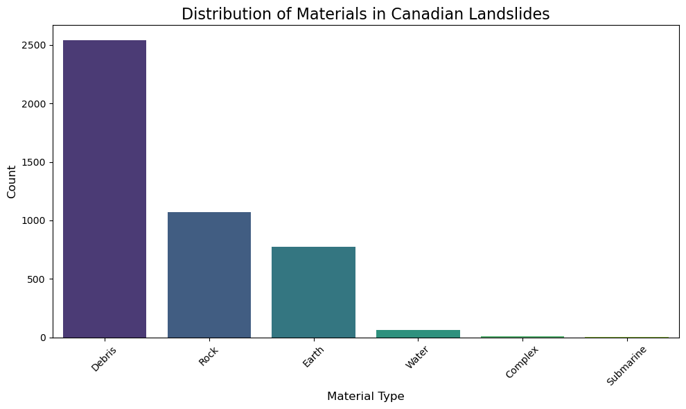
Value counts for 'filter_MATERIAL' (including nulls):
filter_MATERIAL
Debris       2542
Rock         1069
Earth         776
Water          64
Complex         7
Submarine       3
Name: count, dtype: int64
# Plot distribution excluding NaN values
plt.figure(figsize=(10, 6))
non_null_counts = bc_gdf['filter_MATERIAL'].value_counts()
sns.barplot(x=non_null_counts.index, y=non_null_counts.values,
            palette='viridis', hue=non_null_counts.index, legend=False)
plt.title('Distribution of Materials in Canadian Landslides', fontsize=16)
plt.xlabel('Material Type', fontsize=12)
plt.ylabel('Count', fontsize=12)
plt.xticks(rotation=45)
plt.tight_layout()
plt.show()
Extracting Movement from Type#
def extract_movement_class_canada(type_str):
    # Return NaN for empty or null values
    if pd.isna(type_str) or str(type_str).strip() == '':
        return pd.NA

    type_str = str(type_str).lower()

    movement_classes = []

    # Check for complex first
    if 'complex' in type_str:
        movement_classes.append('Complex')

    # Check for slide types
    if 'slide' in type_str:
        movement_classes.append('Slide')

    # Check for flow
    if 'flow' in type_str:
        movement_classes.append('Flow')

    # Check for fall
    if 'fall' in type_str:
        movement_classes.append('Fall')

    # Check for spread
    if 'spread' in type_str:
        movement_classes.append('Spread')

    # Check for topple
    if 'topple' in type_str:
        movement_classes.append('Topple')

    # Check for avalanche
    if 'avalanche' in type_str:
        movement_classes.append('Avalanche')

    # Check for flood
    if 'flood' in type_str or 'glof' in type_str:
        movement_classes.append('Flood')

    # Special cases
    if 'mountain slope deformation' in type_str:
        movement_classes.append('Deformation')
    if 'flowslide' in type_str:
        movement_classes.append('Flow+Slide')
    if 'submarine' in type_str:
        movement_classes.append('Submarine')

    # If no movement class was identified but the string isn't empty
    if not movement_classes:
        return 'Other'

    # Join all identified movement classes with '+'
    return '+'.join(movement_classes)

# Apply the function to create a new column
bc_gdf['filter_MOVEMENT'] = bc_gdf['Type'].apply(extract_movement_class_canada)

print("\nValue counts for 'MOVEMENT':")
movement_counts = bc_gdf['filter_MOVEMENT'].value_counts(dropna=False)
print(movement_counts)
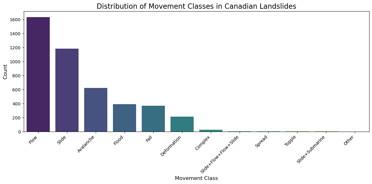
Value counts for 'MOVEMENT':
filter_MOVEMENT
Flow                     1633
Slide                    1181
Avalanche                 623
Flood                     392
Fall                      368
Deformation               215
Complex                    27
Slide+Flow+Flow+Slide       7
Spread                      6
Topple                      4
Slide+Submarine             3
Other                       2
Name: count, dtype: int64
plt.figure(figsize=(12, 6))
non_null_counts = bc_gdf['filter_MOVEMENT'].value_counts()
sns.barplot(x=non_null_counts.index, y=non_null_counts.values,
            palette='viridis', hue=non_null_counts.index, legend=False)
plt.title('Distribution of Movement Classes in Canadian Landslides', fontsize=16)
plt.xlabel('Movement Class', fontsize=12)
plt.ylabel('Count', fontsize=12)
plt.xticks(rotation=45, ha='right')
plt.tight_layout()
plt.show()
# Summary of the new columns
print("Summary of newly created columns:")
print(f"Total records: {len(bc_gdf)}")
print(f"\nOriginal 'Type' column had {bc_gdf['Type'].nunique()} unique values")
print(f"New 'MATERIAL' column has {bc_gdf['filter_MATERIAL'].nunique()} unique values")
print(f"New 'MOVEMENT' column has {bc_gdf['filter_MOVEMENT'].nunique()} unique values")

print(f"\nSample of new columns:")
print(bc_gdf[['Type', 'filter_MATERIAL', 'filter_MOVEMENT']].head(10))
Summary of newly created columns:
Total records: 4461

Original 'Type' column had 22 unique values
New 'MATERIAL' column has 6 unique values
New 'MOVEMENT' column has 12 unique values

Sample of new columns:
                Type filter_MATERIAL filter_MOVEMENT
86  Debris avalanche          Debris       Avalanche
87  Debris avalanche          Debris       Avalanche
88  Debris avalanche          Debris       Avalanche
89  Debris avalanche          Debris       Avalanche
90  Debris avalanche          Debris       Avalanche
91  Debris avalanche          Debris       Avalanche
92  Debris avalanche          Debris       Avalanche
93  Debris avalanche          Debris       Avalanche
94  Debris avalanche          Debris       Avalanche
95  Debris avalanche          Debris       Avalanche
Old Material Class#
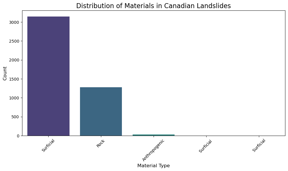
material_counts = bc_gdf['Material'].value_counts(dropna=False)
print("\nValue counts for 'Material':")
print(material_counts)
Value counts for 'Material':
Material
Surficial        3147
Rock             1280
Anthropogenic      28
Surficial           4
 Surficial          2
Name: count, dtype: int64
plt.figure(figsize=(10, 6))
sns.barplot(x=material_counts.index, y=material_counts.values,
            palette='viridis', hue=material_counts.index, legend=False)
plt.title('Distribution of Materials in Canadian Landslides', fontsize=16)
plt.xlabel('Material Type', fontsize=12)
plt.ylabel('Count', fontsize=12)
plt.xticks(rotation=45)
plt.tight_layout()
plt.show()
Size Class#
size_counts = bc_gdf['Size_class'].value_counts(dropna=False)
print("\nValue counts for 'Size_class':")
print(size_counts)
Value counts for 'Size_class':
Size_class
4202
Large 34
Small 25
20Â 9
25Â 7
...
400 1
2000 1
1850 1
380 1
10000-30000 1
Name: count, Length: 134, dtype: int64
Timing#
timing_counts = bc_gdf['Timing'].value_counts(dropna=False)
print("\nValue counts for 'Timing':")
print(timing_counts)
Value counts for 'Timing':
Timing
2212
15-Nov-21 1351
2022-Aug-10 177
July 17; 2022Â 64
2018 59
...
23-01-1958 1
30 Nov -1\nDec 1958 1
29-04-1959 1
27-01-1960 1
4-Mar-22 1
Name: count, Length: 330, dtype: int64
Create a new DataFrame#
bc_gdf.dtypes
LS_ID                          object
Name                           object
Longitude                     float64
Latitude                      float64
Type                           object
Material                       object
Size_class                     object
Timing                         object
Trigger                        object
Contributo                     object
Reference                      object
Type_details                   object
Cont_details                   object
Resource_road_activity         object
Resource_road_type             object
Study_area                     object
Watercours                     object
Event_verification             object
Volume_estimate_method         object
Discharge estimate (m3/s)      object
Deposit_Arrea_m2               object
Bedrock_type                   object
Point_location                 object
Location_confidence            object
Comment                        object
geometry                     geometry
filter_MATERIAL                object
filter_MOVEMENT                object
dtype: object
Possible Mapping
-LS_ID LANDSLIDE_ID
Name NAME
Longitude
Latitude
Type Type in Oregon
Material
Size_class
Timing
Trigger
Contributo
Reference Reference
Type_details
Cont_details
Resource_road_activity
Resource_road_type
Study_area
Watercours
Event_verification
Volume_estimate_method
Discharge estimate (m3/s)
Deposit_Arrea_m2 Area
Bedrock_type
Point_location
Location_confidence confidence
Comment comment
geometry geometry
NEW_MATERIAL Material
MOVEMENT Movement
dtype: object
bc_gdf["filter_CONFIDENCE"] = bc_gdf['Location_confidence']
bc_gdf.dtypes
LS_ID                          object
Name                           object
Longitude                     float64
Latitude                      float64
Type                           object
Material                       object
Size_class                     object
Timing                         object
Trigger                        object
Contributo                     object
Reference                      object
Type_details                   object
Cont_details                   object
Resource_road_activity         object
Resource_road_type             object
Study_area                     object
Watercours                     object
Event_verification             object
Volume_estimate_method         object
Discharge estimate (m3/s)      object
Deposit_Arrea_m2               object
Bedrock_type                   object
Point_location                 object
Location_confidence            object
Comment                        object
geometry                     geometry
filter_MATERIAL                object
filter_MOVEMENT                object
filter_CONFIDENCE              object
dtype: object
bc_gdf['filter_ORIGIN'] = 'BC'
bc_gdf['filter_DATASET_LINK'] = 'https://data.niaid.nih.gov/resources?id=zenodo_7089351'
bc_gdf['filter_REFERENCE'] = bc_gdf['Reference']
Save into GeoJSON#
bc_gdf.to_file("./processed_geojson/bc_landslides.geojson", driver='GeoJSON')
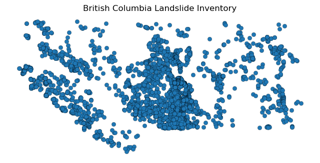
bc_gdf.plot(figsize=(8, 6), edgecolor="k", linewidth=0.2)
plt.title("British Columbia Landslide Inventory")
plt.axis("off")
plt.show()