
GPS/GNSS Time Series Analysis: Fundamentals to Slow Slip Events#
CRESCENT Technical Short Course, Strain Accumulation and Release from GNSS
Day 1: GNSS Time Series Analysis
Created By: Brendan Crowell, The Ohio State University, Chair of C3S Working Group#
Overview#
This extended notebook provides a comprehensive, end-to-end workflow for analyzing GPS/GNSS time series from the Cascadia subduction zone. We will:
Load & inspect CRESCENT netCDF data
Map station networks
Decompose signals into interseismic, coseismic, and seasonal components
Detect slow slip / transient events using RSI + kurtosis
Extract a single slow slip event and measure displacement offsets
Estimate uncertainties on those offsets
Physical context#
The Cascadia subduction zone hosts episodic tremor and slip (ETS) events — periodic slow earthquakes on the deep locked interface. GPS stations show ~5–10 mm transient displacements (opposite to the long-term interseismic direction) with characteristic recurrence of ~14 months. Isolating these signals requires removing:
Interseismic trend — steady plate convergence loading
Seasonal signals — annual/semi-annual cycles from hydrology & thermal loading
Coseismic offsets — instantaneous jumps from earthquakes
After removing these, the residual reveals the slow slip signature.
1. Environment Setup#
Import all libraries needed throughout the notebook.
import numpy as np
import xarray as xr
import matplotlib.pyplot as plt
import matplotlib.dates as mdates
from matplotlib.gridspec import GridSpec
import pandas as pd
import calendar
import math
import warnings
warnings.filterwarnings('ignore')

from scipy import stats
from scipy.signal import detrend
from scipy.stats import kurtosis
from scipy.special import erf
from scipy.optimize import curve_fit, least_squares
from scipy.linalg import lstsq

# Plotting defaults for publication-quality figures
plt.rcParams.update({
    'figure.dpi': 120,
    'font.size': 11,
    'axes.labelsize': 12,
    'axes.titlesize': 13,
    'lines.linewidth': 1.2,
    'legend.fontsize': 10,
})

print("All libraries loaded successfully.")
All libraries loaded successfully.
2. Loading the CRESCENT GNSS Dataset#
The CRESCENT project provides three independently processed GPS time series datasets:
Provider |
Description |
|---|---|
SOPAC |
Scripps Orbit and Permanent Array Center |
PANGA |
Pacific Northwest Geodetic Array |
UNR |
University of Nevada, Reno Nevada Geodetic Lab |
All three are provided in a unified netCDF format with identical variable names, allowing algorithm comparison across solutions. The UNR data is in the North American fixed reference frame whereas the SOPAC/PANGA solutions are in ITRF. The reference frame here matters when modeling the long term interseismic signals, but can be easily corrected with an Euler pole rotation. Also, double-check the units since it may be mm or meters; the interseismic velocities should be 10s of mm/yr.
import requests
from io import BytesIO

# ── Choose your data provider ──────────────────────────────────────────────
# Uncomment the URL for the dataset you want to use

# SOPAC data
url = "https://zenodo.org/records/20518159/files/gnss_SOPAC_trend_2010_2025.nc?download=1"

# PANGA data
#url = "https://zenodo.org/records/20518159/files/gnss_PANGA_trend_2010_2025.nc?download=1"

# UNR data
#url = "https://zenodo.org/records/19616474/files/gnss_unr_2010_2025.nc?download=1"

print(f"Downloading dataset...")
response = requests.get(url)
response.raise_for_status()

ds = xr.open_dataset(BytesIO(response.content), engine="h5netcdf")
print("Dataset loaded successfully!")
print(ds)
Downloading dataset...
Dataset loaded successfully!
<xarray.Dataset> Size: 111MB
Dimensions:        (station: 340, time: 5844)
Coordinates:
  * station        (station) <U4 5kB 'albh' 'arli' 'asbu' ... 'yelm' 'yonc'
  * time           (time) datetime64[ns] 47kB 2010-01-01 ... 2025-12-31
    lat            (station) float64 3kB ...
    lon            (station) float64 3kB ...
    elev_m         (station) float64 3kB ...
Data variables:
    dec_year       (station, time) float64 16MB ...
    east_m         (station, time) float64 16MB ...
    north_m        (station, time) float64 16MB ...
    up_m           (station, time) float64 16MB ...
    east_sigma_m   (station, time) float64 16MB ...
    north_sigma_m  (station, time) float64 16MB ...
    up_sigma_m     (station, time) float64 16MB ...
3. Dataset Inspection#
Before analysis, it is critical to understand the structure and content of the dataset.
# ── Dataset dimensions and coordinates ───────────────────────────────────
print("=== Dataset Dimensions ===")
for dim, size in ds.dims.items():
    print(f"  {dim}: {size}")

print("\n=== Coordinates ===")
for coord in ds.coords:
    print(f"  {coord}: {ds[coord].dims}, dtype={ds[coord].dtype}")

print("\n=== Data Variables ===")
for var in ds.data_vars:
    print(f"  {var}: {ds[var].dims}, dtype={ds[var].dtype}, units={ds[var].attrs.get('units','?')}")
=== Dataset Dimensions ===
  station: 340
  time: 5844

=== Coordinates ===
  time: ('time',), dtype=datetime64[ns]
  station: ('station',), dtype=<U4
  lat: ('station',), dtype=float64
  lon: ('station',), dtype=float64
  elev_m: ('station',), dtype=float64

=== Data Variables ===
  dec_year: ('station', 'time'), dtype=float64, units=?
  east_m: ('station', 'time'), dtype=float64, units=?
  north_m: ('station', 'time'), dtype=float64, units=?
  up_m: ('station', 'time'), dtype=float64, units=?
  east_sigma_m: ('station', 'time'), dtype=float64, units=?
  north_sigma_m: ('station', 'time'), dtype=float64, units=?
  up_sigma_m: ('station', 'time'), dtype=float64, units=?
# ── Station metadata ──────────────────────────────────────────────────────
station_lat  = ds.lat.values
station_lon  = ds.lon.values
station_elev = ds.elev_m.values
station_names = ds.station.values

print(f"Number of stations : {len(station_names)}")
print(f"Latitude range     : {np.nanmin(station_lat):.2f}° – {np.nanmax(station_lat):.2f}°N")
print(f"Longitude range    : {np.nanmin(station_lon):.2f}° – {np.nanmax(station_lon):.2f}°E")
print(f"Elevation range    : {np.nanmin(station_elev):.0f} – {np.nanmax(station_elev):.0f} m")
print(f"\nFirst 10 station names: {station_names[:10]}")
Number of stations : 340
Latitude range     : 39.53° – 50.64°N
Longitude range    : -128.13° – -121.05°E
Elevation range    : -22 – 3068 m

First 10 station names: ['albh' 'arli' 'asbu' 'ashl' 'bamf' 'bcov' 'beli' 'bend' 'bils' 'bly1']
4. Station Network Map#
Visualizing the spatial distribution of the network helps identify regional coverage and select stations for detailed analysis. The CRESCENT dataset selected specific lat/lon boundaries and excluded sites with less than 5 years of data. More continuous stations exist if you check UNR’s geodesy lab map (https://geodesy.unr.edu/NGLStationPages/gpsnetmap/GPSNetMap.html).
ds_plot = ds.where(ds.lon.notnull() & ds.lat.notnull(), drop=True)
n_total = ds.sizes["station"]
n_ok    = ds_plot.sizes["station"]

fig, ax = plt.subplots(figsize=(10, 8))

sc = ax.scatter(ds_plot.lon, ds_plot.lat, s=18, c=ds_plot.elev_m,
                cmap='terrain', alpha=0.85, edgecolors='k', linewidths=0.3)

# Highlight the primary analysis station (ALBH)
albh_lat = float(ds.sel(station="albh").lat)
albh_lon = float(ds.sel(station="albh").lon)
ax.scatter(albh_lon, albh_lat, s=120, c='red', marker='*',
           zorder=5, label='ALBH (primary analysis station)')

cbar = fig.colorbar(sc, ax=ax, shrink=0.8)
cbar.set_label("Elevation (m)")

ax.set_xlabel("Longitude (°E)")
ax.set_ylabel("Latitude (°N)")
ax.set_title(f"GNSS Station Network — Cascadia Subduction Zone\n({n_ok}/{n_total} stations with valid coordinates)")
ax.legend(loc='lower left')
ax.grid(True, alpha=0.4)
ax.set_aspect("equal", adjustable="box")
plt.tight_layout()
plt.show()
print(f"Map shows {n_ok} stations with valid coordinates out of {n_total} total.")
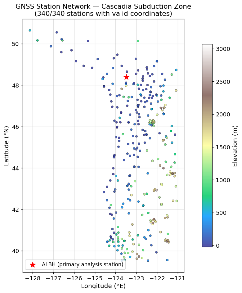
Map shows 340 stations with valid coordinates out of 340 total.
5. Single Station Inspection: ALBH#
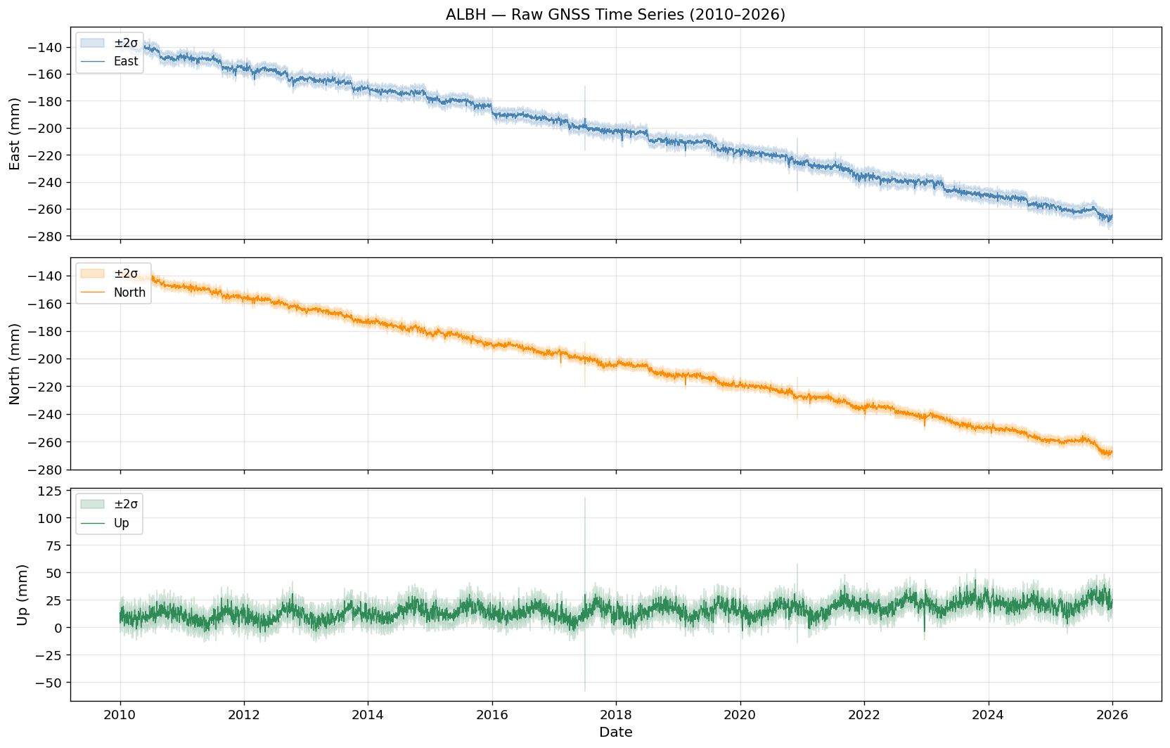
Station ALBH (Albert Head, British Columbia) is one of the best-characterized continuous GPS sites in Cascadia, with a long record showing multiple well-documented ETS events. This is one of stations in the original ETS paper by Rogers and Dragert. We load all three displacement components (East, North, Up) and their uncertainties. The trend that will be shown in the SOPAC solutions are in the ITRF frame.
# ── Load ALBH ────────────────────────────────────────────────────────────
stat = ds.sel(station="albh")

df_albh = pd.DataFrame({
    'time'      : pd.to_datetime(stat.time.values),
    'dec_year'  : stat.dec_year.values,
    'east_mm'   : stat.east_m.values  * 1000,
    'north_mm'  : stat.north_m.values * 1000,
    'up_mm'     : stat.up_m.values    * 1000,
    'east_sig'  : stat.east_sigma_m.values  * 1000,
    'north_sig' : stat.north_sigma_m.values * 1000,
    'up_sig'    : stat.up_sigma_m.values    * 1000,
})

print(f"Station ALBH — {df_albh.shape[0]} daily observations")
print(f"Date range   : {df_albh.time.min().date()} → {df_albh.time.max().date()}")
print(f"\nData availability:")
for col in ['east_mm','north_mm','up_mm']:
    n_valid = df_albh[col].notna().sum()
    pct = 100*n_valid/len(df_albh)
    print(f"  {col:12s}: {n_valid:5d} valid ({pct:.1f}%)")

df_albh.head(10)
Station ALBH — 5844 daily observations
Date range   : 2010-01-01 → 2025-12-31

Data availability:
  east_mm     :  5833 valid (99.8%)
  north_mm    :  5833 valid (99.8%)
  up_mm       :  5833 valid (99.8%)
| time | dec_year | east_mm | north_mm | up_mm | east_sig | north_sig | up_sig | |
|---|---|---|---|---|---|---|---|---|
| 0 | 2010-01-01 | 2010.0014 | -136.79 | -137.65 | 13.17 | 2.12 | 1.53 | 4.90 |
| 1 | 2010-01-02 | 2010.0041 | -137.49 | -137.65 | 10.07 | 1.85 | 1.40 | 4.39 |
| 2 | 2010-01-03 | 2010.0068 | -137.29 | -136.65 | 3.87 | 1.72 | 1.40 | 4.26 |
| 3 | 2010-01-04 | 2010.0096 | -137.99 | -136.85 | 13.07 | 1.72 | 1.40 | 4.26 |
| 4 | 2010-01-05 | 2010.0123 | -138.19 | -136.65 | 13.47 | 1.99 | 1.40 | 4.51 |
| 5 | 2010-01-06 | 2010.0151 | -137.29 | -137.25 | 9.97 | 1.85 | 1.40 | 4.64 |
| 6 | 2010-01-07 | 2010.0178 | -137.89 | -137.75 | 6.37 | 1.99 | 1.40 | 4.64 |
| 7 | 2010-01-08 | 2010.0205 | -137.39 | -138.95 | 14.47 | 2.38 | 1.66 | 5.03 |
| 8 | 2010-01-09 | 2010.0233 | -137.29 | -139.45 | 15.27 | 1.99 | 1.53 | 4.64 |
| 9 | 2010-01-10 | 2010.0260 | -138.59 | -138.75 | 9.17 | 2.25 | 1.53 | 4.90 |
# ── Full record 3-component plot ─────────────────────────────────────────
fig, axes = plt.subplots(3, 1, figsize=(14, 9), sharex=True)
components = [('east_mm', 'East',  'steelblue'),
              ('north_mm', 'North', 'darkorange'),
              ('up_mm',    'Up',    'seagreen')]

for ax, (col, label, color) in zip(axes, components):
    sig_col = col.replace('_mm','_sig')
    ax.fill_between(df_albh.time,
                    df_albh[col] - 2*df_albh[sig_col],
                    df_albh[col] + 2*df_albh[sig_col],
                    alpha=0.2, color=color, label='±2σ')
    ax.plot(df_albh.time, df_albh[col], color=color, lw=0.8, label=label)
    ax.set_ylabel(f"{label} (mm)")
    ax.grid(True, alpha=0.3)
    ax.legend(loc='upper left')

axes[0].set_title("ALBH — Raw GNSS Time Series (2010–2026)")
axes[2].set_xlabel("Date")
plt.tight_layout()
plt.show()
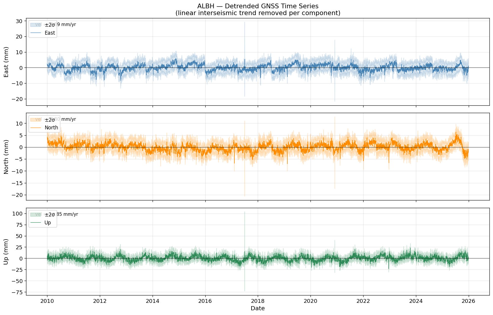
# ── Detrended 3-component plot ────────────────────────────────────────────
# Fits offset + velocity + annual + semi-annual per component using numpy
# lstsq, then removes the linear trend. No external functions required.
from numpy.linalg import lstsq as np_lstsq

fig, axes = plt.subplots(3, 1, figsize=(14, 9), sharex=True)
components = [('east_mm', 'East',  'steelblue'),
              ('north_mm', 'North', 'darkorange'),
              ('up_mm',    'Up',    'seagreen')]

t = df_albh.dec_year.values

# Design matrix: offset + trend + annual cos/sin + semi-annual cos/sin
G = np.column_stack([
    np.ones(len(t)),
    t,
    np.cos(2*np.pi*t),
    np.sin(2*np.pi*t),
    np.cos(4*np.pi*t),
    np.sin(4*np.pi*t),
])

for ax, (col, label, color) in zip(axes, components):
    sig_col = col.replace('_mm','_sig')
    d = df_albh[col].values
    sig = df_albh[sig_col].values

    # Fit on valid observations only
    valid = ~np.isnan(d) & ~np.isnan(sig) & (sig > 0)
    m, _, _, _ = np_lstsq(G[valid], d[valid], rcond=None)

    # Remove only the linear trend (offset + velocity)
    trend = m[0] + m[1]*t
    detrended = df_albh[col] - trend

    ax.fill_between(df_albh.time,
                    detrended - 2*df_albh[sig_col],
                    detrended + 2*df_albh[sig_col],
                    alpha=0.2, color=color, label='±2σ')
    ax.plot(df_albh.time, detrended, color=color, lw=0.8, label=label)
    ax.set_ylabel(f"{label} (mm)")
    ax.axhline(0, color='k', lw=0.5)
    ax.grid(True, alpha=0.3)
    ax.legend(loc='upper left')
    ax.text(0.02, 0.95, f"vel = {m[1]:+.2f} mm/yr",
            transform=ax.transAxes, fontsize=9, va='top')

axes[0].set_title("ALBH — Detrended GNSS Time Series\n"
                  "(linear interseismic trend removed per component)")
axes[2].set_xlabel("Date")
plt.tight_layout()
plt.show()
6. Signal Decomposition Model#
GPS time series are conventionally modeled as a superposition of several deterministic signals:
where:
\(a\) = constant offset (reference position)
\(b\) = interseismic (secular) velocity (mm/yr)
\(H(t - t_k^{co})\) = Heaviside step function at coseismic time \(t_k^{co}\)
\(c_k\) = coseismic offset magnitude
\(A_{ann}, B_{ann}\) = annual sine/cosine amplitudes
\(A_{semi}, B_{semi}\) = semi-annual sine/cosine amplitudes
\(r(t)\) = residual (contains slow slip, noise)
The design matrix approach makes this a linear inverse problem, solvable by weighted least squares. For large coseismic events, a postseismic decay term would have a similar form to the coseismic terms (with a Heaviside step function) except with an exponental or logarithmic decay (the decay coefficient will need to be solved for through a grid search).
def build_design_matrix(dec_year, coseismic_times=None):
    """
    Build the least-squares design matrix G such that d = G @ m + noise.

    Columns:
      0 : constant (offset)
      1 : linear trend (interseismic velocity)
      2 : cos(2π t)  — annual cosine
      3 : sin(2π t)  — annual sine
      4 : cos(4π t)  — semi-annual cosine
      5 : sin(4π t)  — semi-annual sine
      6+ : Heaviside step functions for each coseismic epoch

    Parameters
    ----------
    dec_year        : array of decimal years
    coseismic_times : list of decimal year epochs for coseismic steps

    Returns
    -------
    G : (n, m) design matrix
    col_names : list of column descriptions
    """
    t = dec_year
    n = len(t)

    # Base columns: offset + trend + annual + semi-annual
    G = np.column_stack([
        np.ones(n),                    # offset
        t,                             # trend (velocity)
        np.cos(2 * np.pi * t),         # annual cos
        np.sin(2 * np.pi * t),         # annual sin
        np.cos(4 * np.pi * t),         # semi-annual cos
        np.sin(4 * np.pi * t),         # semi-annual sin
    ])
    col_names = ['offset', 'velocity', 'annual_cos', 'annual_sin',
                 'semiann_cos', 'semiann_sin']

    # Add Heaviside steps for coseismic epochs
    if coseismic_times:
        for t_co in coseismic_times:
            step = (t >= t_co).astype(float)
            G = np.column_stack([G, step])
            col_names.append(f'coseis_{t_co:.3f}')

    return G, col_names


def fit_model(dec_year, displacement_mm, sigma_mm=None, coseismic_times=None):
    """
    Fit the GPS signal decomposition model using weighted least squares.

    Returns a dict with:
      model_params, param_names, param_std, residuals,
      trend, seasonal, coseismic, full_fit
    """
    # Remove NaN observations
    valid = ~np.isnan(displacement_mm)
    if sigma_mm is not None:
        valid &= ~np.isnan(sigma_mm) & (sigma_mm > 0)

    t_v = dec_year[valid]
    d_v = displacement_mm[valid]

    G, col_names = build_design_matrix(t_v, coseismic_times)

    # Weight matrix: W = diag(1/sigma^2)
    if sigma_mm is not None:
        w = 1.0 / sigma_mm[valid]**2
        W = np.diag(w)
        # Weighted least squares: m = (G^T W G)^{-1} G^T W d
        GTW   = G.T @ W
        GTWGi = np.linalg.pinv(GTW @ G)
        m     = GTWGi @ GTW @ d_v
        # Formal covariance
        Cm = GTWGi
    else:
        m, _, _, _ = lstsq(G, d_v)
        GTG = G.T @ G
        Cm  = np.linalg.pinv(GTG) * np.var(d_v - G @ m)

    m_std = np.sqrt(np.diag(Cm))

    # Reconstruct model terms over the full time axis
    G_full, _ = build_design_matrix(dec_year, coseismic_times)
    fit_full = G_full @ m

    trend = G_full[:, 0] * m[0] + G_full[:, 1] * m[1]          # offset + velocity
    seasonal = (G_full[:, 2] * m[2] + G_full[:, 3] * m[3] +     # annual
                G_full[:, 4] * m[4] + G_full[:, 5] * m[5])       # + semi-annual

    coseis_fit = np.zeros(len(dec_year))
    if coseismic_times and len(col_names) > 6:
        for i, t_co in enumerate(coseismic_times):
            coseis_fit += G_full[:, 6+i] * m[6+i]

    residuals = displacement_mm - fit_full

    return {
        'params'     : m,
        'param_names': col_names,
        'param_std'  : m_std,
        'fit'        : fit_full,
        'trend'      : trend,
        'seasonal'   : seasonal,
        'coseismic'  : coseis_fit,
        'residuals'  : residuals,
        'valid_mask' : valid,
    }

print("Design matrix functions defined.")
print("Model: d(t) = offset + velocity·t + annual + semi-annual + Σ coseismic steps")
Design matrix functions defined.
Model: d(t) = offset + velocity·t + annual + semi-annual + Σ coseismic steps
7. Fit the Full Decomposition Model#
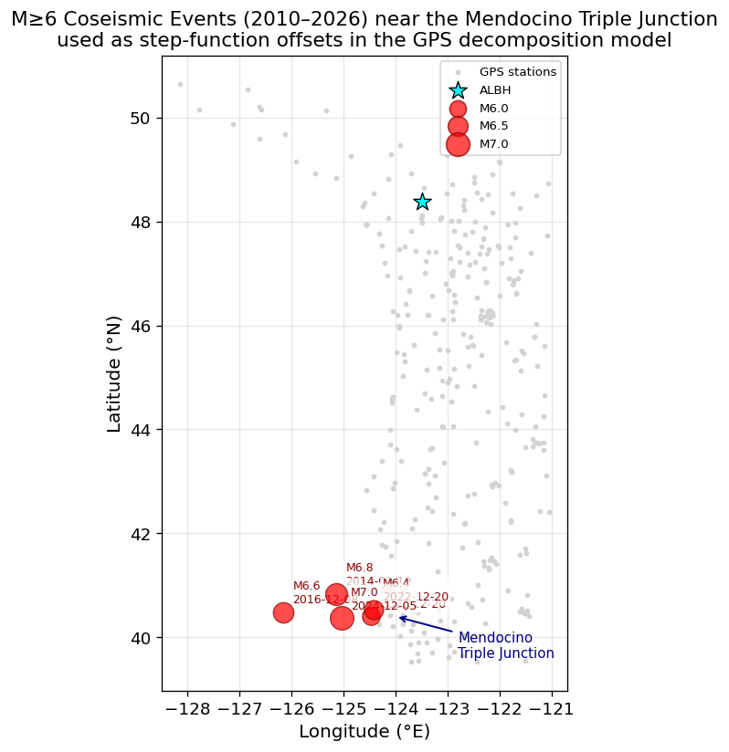
We fit the model to all three components. The coseismic step terms handle instantaneous offsets from large earthquakes. Here we include significant M≥6 earthquakes near the Mendocino Triple Junction (the southern terminus of the Cascadia subduction zone) that have occurred between 2010 and 2026 and are known to produce measurable static offsets at GPS stations throughout northern California and southern Oregon. Details of the earthquake catalog are defined in the cell below. Note that for stations far away, like ALBH, the coseismic offsets from Mendocino earthquakes will be negligible, but we include them here to simply demonstrate the model term determination.
# ══════════════════════════════════════════════════════════════════
# COSEISMIC EPOCH CATALOG — Mendocino Triple Junction M≥6 (2010–2026)
# Sources: USGS ComCat
# ══════════════════════════════════════════════════════════════════

import pandas as pd

# Each entry: (ISO date string, magnitude, description, lat, lon, depth_km)
mendocino_catalog = [
    # 2014-03-10 M6.8 — Gorda plate intraplate, left-lateral strike-slip
    # 78 km WNW of Ferndale, CA; USGS nc72182046
    ("2014-03-10", 6.8, "Gorda plate intraplate — left-lateral strike-slip, "
     "78 km WNW of Ferndale",
     40.83, -125.13, 16.4),

    # 2016-12-08 M6.6 — Offshore Cape Mendocino, Mendocino Transform Fault
    ("2016-12-08", 6.6, "Offshore Cape Mendocino — Mendocino Transform Fault (right-lateral)",
     40.48, -126.15, 10.0),

    # 2021-12-20 M6.2 (two events: M6.1 + M6.0 within 11 s) — Petrolia, Gorda slab
    ("2021-12-20", 6.2, "Petrolia — Gorda plate intraplate (two events ~11 s apart, M6.1+M6.0)",
     40.40, -124.47, 27.0),

    # 2022-12-20 M6.4 — Offshore Ferndale, Gorda plate left-lateral strike-slip
    ("2022-12-20", 6.4, "Offshore Ferndale — Gorda plate intraplate (left-lateral strike-slip)",
     40.53, -124.42, 16.0),

    # 2024-12-05 M7.0 — Offshore Cape Mendocino, Mendocino Transform Fault
    ("2024-12-05", 7.0, "Offshore Cape Mendocino — Mendocino Transform Fault M7.0 (right-lateral)",
     40.37, -125.03, 10.0),
]

# Build decimal-year epoch list
def date_to_dec_year(date_str):
    """Convert ISO date string to decimal year."""
    dt = pd.Timestamp(date_str)
    year_start = pd.Timestamp(f'{dt.year}-01-01')
    year_end   = pd.Timestamp(f'{dt.year+1}-01-01')
    frac = (dt - year_start).total_seconds() / (year_end - year_start).total_seconds()
    return dt.year + frac

cat_df = pd.DataFrame(mendocino_catalog,
                      columns=['date','mag','description','lat','lon','depth_km'])
cat_df['dec_year'] = cat_df['date'].apply(date_to_dec_year)

print("Mendocino Triple Junction Coseismic Catalog (M≥6, 2010–2026)")
print("=" * 80)
for _, row in cat_df.iterrows():
    print(f"  {row['date'][:10]}  M{row['mag']:.1f}  t={row['dec_year']:.4f}")
    print(f"    {row['description']}")
    print(f"    Location: {row['lat']:.3f}°N, {row['lon']:.3f}°E, depth={row['depth_km']:.0f} km")
    print()

# ── Extract unique daily-resolution epochs for the model ─────────────────
# The M7.0 and M6.6 both fall on 2024-12-05 at daily resolution → keep only one
unique_epochs = []
seen_dates = set()
for _, row in cat_df.sort_values('mag', ascending=False).iterrows():
    day_str = str(row['date'])[:10]
    if day_str not in seen_dates:
        seen_dates.add(day_str)
        unique_epochs.append(date_to_dec_year(day_str))

unique_epochs = sorted(unique_epochs)
print(f"Unique daily-resolution epochs for GPS step model: {len(unique_epochs)}")
for e in unique_epochs:
    print(f"  {e:.4f}")

dec_year = df_albh.dec_year.values

print("\nFitting interseismic + seasonal + coseismic model to all 3 components...")
results = {}
for comp, label in [('east_mm','East'), ('north_mm','North'), ('up_mm','Up')]:
    sig_col = comp.replace('_mm','_sig')
    results[comp] = fit_model(
        dec_year,
        df_albh[comp].values,
        sigma_mm=df_albh[sig_col].values,
        coseismic_times=unique_epochs
    )

# ── Print fitted parameters ───────────────────────────────────────────────
for comp, label in [('east_mm','East'), ('north_mm','North'), ('up_mm','Up')]:
    r = results[comp]
    print(f"\n{'='*55}")
    print(f"{label} Component — Fitted Parameters")
    print(f"{'='*55}")
    for name, val, std in zip(r['param_names'], r['params'], r['param_std']):
        print(f"  {name:25s}: {val:+10.4f}  ±{std:.4f}")
    valid = r['valid_mask']
    res_mm = r['residuals'][valid]
    print(f"  {'RMS residual':25s}: {np.sqrt(np.nanmean(res_mm**2)):.3f} mm")

# Alias for downstream cells
COSEISMIC_EPOCHS = unique_epochs
all_steps = unique_epochs
Mendocino Triple Junction Coseismic Catalog (M≥6, 2010–2026)
================================================================================
  2014-03-10  M6.8  t=2014.1863
    Gorda plate intraplate — left-lateral strike-slip, 78 km WNW of Ferndale
    Location: 40.830°N, -125.130°E, depth=16 km

  2016-12-08  M6.6  t=2016.9344
    Offshore Cape Mendocino — Mendocino Transform Fault (right-lateral)
    Location: 40.480°N, -126.150°E, depth=10 km

  2021-12-20  M6.2  t=2021.9671
    Petrolia — Gorda plate intraplate (two events ~11 s apart, M6.1+M6.0)
    Location: 40.400°N, -124.470°E, depth=27 km

  2022-12-20  M6.4  t=2022.9671
    Offshore Ferndale — Gorda plate intraplate (left-lateral strike-slip)
    Location: 40.530°N, -124.420°E, depth=16 km

  2024-12-05  M7.0  t=2024.9262
    Offshore Cape Mendocino — Mendocino Transform Fault M7.0 (right-lateral)
    Location: 40.370°N, -125.030°E, depth=10 km

Unique daily-resolution epochs for GPS step model: 5
  2014.1863
  2016.9344
  2021.9671
  2022.9671
  2024.9262

Fitting interseismic + seasonal + coseismic model to all 3 components...

=======================================================
East Component — Fitted Parameters
=======================================================
  offset                   : +15542.3690  ±50.2563
  velocity                 :    -7.8020  ±0.0250
  annual_cos               :    -0.4319  ±0.0387
  annual_sin               :    +0.2096  ±0.0391
  semiann_cos              :    +0.4220  ±0.0386
  semiann_sin              :    +0.0943  ±0.0386
  coseis_2014.186          :    +0.6024  ±0.1213
  coseis_2016.934          :    -0.6167  ±0.1261
  coseis_2021.967          :    -1.2543  ±0.1476
  coseis_2022.967          :    +0.4827  ±0.1443
  coseis_2024.926          :    -0.3630  ±0.1364
  RMS residual             : 1.774 mm

=======================================================
North Component — Fitted Parameters
=======================================================
  offset                   : +15499.8201  ±35.9972
  velocity                 :    -7.7812  ±0.0179
  annual_cos               :    -0.7203  ±0.0276
  annual_sin               :    +0.7689  ±0.0279
  semiann_cos              :    +0.0027  ±0.0276
  semiann_sin              :    +0.2173  ±0.0276
  coseis_2014.186          :    -1.5989  ±0.0873
  coseis_2016.934          :    +0.6948  ±0.0906
  coseis_2021.967          :    +0.8480  ±0.1037
  coseis_2022.967          :    -0.6072  ±0.1009
  coseis_2024.926          :    +0.0794  ±0.0955
  RMS residual             : 1.271 mm

=======================================================
Up Component — Fitted Parameters
=======================================================
  offset                   : -1339.1315  ±107.9567
  velocity                 :    +0.6706  ±0.0537
  annual_cos               :    +0.0818  ±0.0825
  annual_sin               :    -4.6083  ±0.0835
  semiann_cos              :    -0.1765  ±0.0825
  semiann_sin              :    +0.8207  ±0.0824
  coseis_2014.186          :    +1.2462  ±0.2647
  coseis_2016.934          :    -1.7635  ±0.2712
  coseis_2021.967          :    +3.6587  ±0.3034
  coseis_2022.967          :    +0.2965  ±0.2952
  coseis_2024.926          :    -0.9287  ±0.2812
  RMS residual             : 4.229 mm
# ══════════════════════════════════════════════════════════════════
# MAP OF MENDOCINO TRIPLE JUNCTION COSEISMIC CATALOG
# ══════════════════════════════════════════════════════════════════

fig, ax = plt.subplots(figsize=(10, 7))

# Station network background
ax.scatter(ds_plot.lon, ds_plot.lat, s=6, c='lightgray', zorder=2, label='GPS stations')

# Earthquake catalog — size scaled to magnitude
for _, row in cat_df.iterrows():
    ms = 2 ** (row['mag'] - 5.0) * 60   # exponential size scaling
    ax.scatter(row['lon'], row['lat'], s=ms,
               c='red', alpha=0.7, edgecolors='darkred', linewidths=0.8,
               zorder=5)
    ax.annotate(f"M{row['mag']:.1f}\n{str(row['date'])[:10]}",
                (row['lon'], row['lat']),
                xytext=(6, 6), textcoords='offset points',
                fontsize=7.5, color='darkred',
                bbox=dict(boxstyle='round,pad=0.2', fc='white', alpha=0.7, lw=0))

# ALBH station
ax.scatter(albh_lon, albh_lat, s=150, c='cyan', marker='*',
           edgecolors='k', linewidths=0.8, zorder=6, label='ALBH')

# Legend for magnitude scale
for m in [6.0, 6.5, 7.0]:
    ax.scatter([], [], s=2**(m-5.0)*60, c='red', alpha=0.7,
               edgecolors='darkred', label=f'M{m:.1f}')

# Mark approximate location of Triple Junction
ax.annotate('Mendocino\nTriple Junction', (-124.0, 40.4),
            xytext=(-122.8, 39.6), textcoords='data',
            fontsize=9, color='navy',
            arrowprops=dict(arrowstyle='->', color='navy', lw=1.2))

ax.set_xlabel("Longitude (°E)")
ax.set_ylabel("Latitude (°N)")
ax.set_title("M≥6 Coseismic Events (2010–2026) near the Mendocino Triple Junction\n"
             "used as step-function offsets in the GPS decomposition model")
ax.legend(loc='upper right', fontsize=8)
ax.grid(True, alpha=0.3)
ax.set_aspect('equal', adjustable='box')
plt.tight_layout()
plt.show()
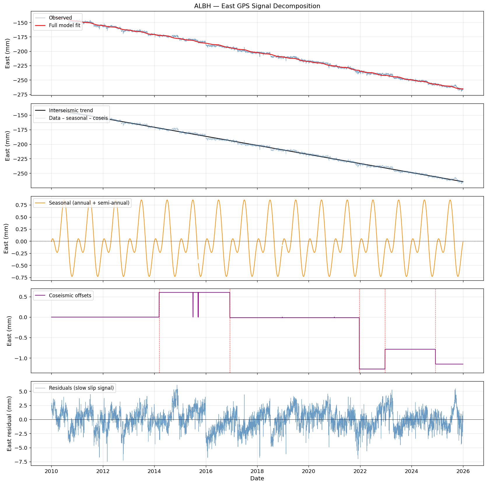
# ── Decomposition plot (East component) ──────────────────────────────────
comp = 'east_mm'
r = results[comp]
t = df_albh.time
label = "East"

fig, axes = plt.subplots(5, 1, figsize=(14, 14), sharex=True)

# 1. Raw data + full fit
axes[0].plot(t, df_albh[comp], 'steelblue', lw=0.7, alpha=0.7, label='Observed')
axes[0].plot(t, r['fit'], 'r-', lw=1.5, label='Full model fit')
axes[0].set_ylabel("East (mm)")
axes[0].set_title(f"ALBH — {label} GPS Signal Decomposition")
axes[0].legend(loc='upper left')

# 2. Interseismic trend
axes[1].plot(t, r['trend'], 'k-', lw=1.5, label='Interseismic trend')
axes[1].plot(t, df_albh[comp] - r['seasonal'] - r['coseismic'],
             'steelblue', lw=0.5, alpha=0.5, label='Data – seasonal – coseis')
axes[1].set_ylabel("East (mm)")
axes[1].legend(loc='upper left')

# 3. Seasonal signal
axes[2].plot(t, r['seasonal'], 'darkorange', lw=1.2, label='Seasonal (annual + semi-annual)')
axes[2].axhline(0, color='k', lw=0.5, ls='--')
axes[2].set_ylabel("East (mm)")
axes[2].legend(loc='upper left')

# 4. Coseismic steps
axes[3].plot(t, r['coseismic'], 'purple', lw=1.2, label='Coseismic offsets')
for t_co in unique_epochs:
    dt = pd.Timestamp(f'{int(t_co)}-01-01') + pd.Timedelta(days=(t_co % 1) * 365.25)
    axes[3].axvline(dt, color='red', ls='--', lw=0.8, alpha=0.7)
axes[3].set_ylabel("East (mm)")
axes[3].legend(loc='upper left')

# 5. Residuals (contains slow slip)
axes[4].plot(t, r['residuals'], 'steelblue', lw=0.7, alpha=0.8, label='Residuals (slow slip signal)')
axes[4].axhline(0, color='k', lw=0.5)
axes[4].set_ylabel("East residual (mm)")
axes[4].set_xlabel("Date")
axes[4].legend(loc='upper left')

for ax in axes:
    ax.grid(True, alpha=0.3)

plt.tight_layout()
plt.show()
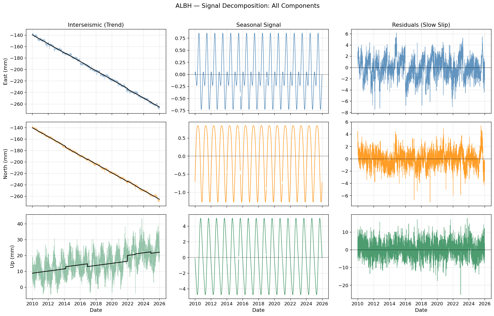
# ── Decomposition for all 3 components side-by-side ─────────────────────
fig, axes = plt.subplots(3, 3, figsize=(16, 10), sharex=True)
t = df_albh.time

titles = ['Interseismic (Trend)', 'Seasonal Signal', 'Residuals (Slow Slip)']
comp_info = [
    ('east_mm',  'East',  'steelblue'),
    ('north_mm', 'North', 'darkorange'),
    ('up_mm',    'Up',    'seagreen'),
]

for row, (comp, label, color) in enumerate(comp_info):
    r = results[comp]

    # Column 0: Trend
    axes[row,0].plot(t, df_albh[comp], color=color, lw=0.6, alpha=0.5)
    axes[row,0].plot(t, r['trend'] + r['coseismic'], 'k-', lw=1.5, label='Trend+coseis')
    axes[row,0].set_ylabel(f"{label} (mm)")

    # Column 1: Seasonal
    axes[row,1].plot(t, r['seasonal'], color=color, lw=1.0)
    axes[row,1].axhline(0, color='k', lw=0.5, ls='--')

    # Column 2: Residuals
    axes[row,2].plot(t, r['residuals'], color=color, lw=0.7, alpha=0.85)
    axes[row,2].axhline(0, color='k', lw=0.5)

for j, title in enumerate(titles):
    axes[0,j].set_title(title)

for ax in axes[-1]:
    ax.set_xlabel("Date")

for ax in axes.flat:
    ax.grid(True, alpha=0.3)

plt.suptitle("ALBH — Signal Decomposition: All Components", fontsize=14, y=1.01)
plt.tight_layout()
plt.show()
8. Seasonal Signal Analysis#
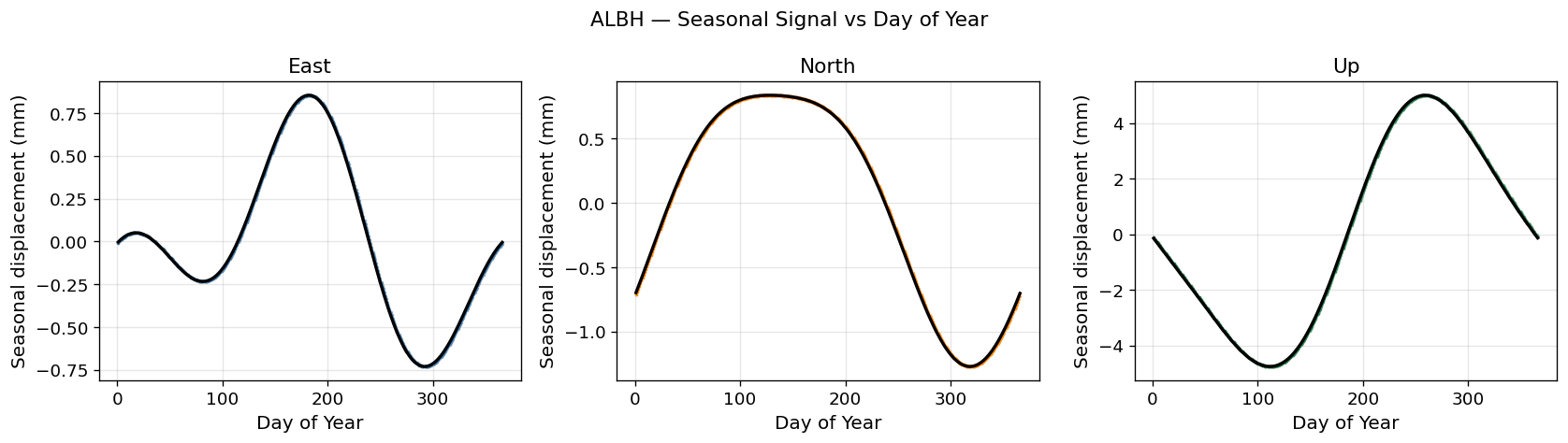
The annual and semi-annual terms capture loading from snow/ice hydrology, atmospheric pressure, and thermal expansion of the crust. Understanding their amplitude and phase is important for correctly isolating transient signals.
# ── Annual cycle: Amplitude and phase ────────────────────────────────────
print(f"{'Component':<10} {'A_ann (mm)':<14} {'B_ann (mm)':<14} {'Amplitude (mm)':<16} {'Phase (DOY)':<12}")
print("-" * 70)

for comp, label, _ in comp_info:
    r = results[comp]
    m = r['params']
    # Columns 2,3 = annual cos, sin
    A = m[2]; B = m[3]
    amplitude = np.sqrt(A**2 + B**2)
    # Phase: peak displacement occurs at phase_yr (fraction of year from Jan 1)
    phase_yr  = -np.arctan2(B, A) / (2 * np.pi)  # fractional year
    phase_doy = phase_yr % 1.0 * 365.25
    print(f"{label:<10} {A:+.4f}        {B:+.4f}        {amplitude:.4f}          {phase_doy:.1f}")

print()
# ── Plot seasonal signal vs DOY ───────────────────────────────────────────
fig, axes = plt.subplots(1, 3, figsize=(14, 4), sharey=False)
for ax, (comp, label, color) in zip(axes, comp_info):
    r = results[comp]
    # Extract DOY
    doy = df_albh.time.dt.dayofyear.values
    ax.scatter(doy, r['seasonal'], s=1, c=color, alpha=0.2)

    # Overplot model curve
    t_doy = np.linspace(1, 366, 366)
    t_yr  = 2015 + t_doy/365.25          # arbitrary year, only fractional part matters
    A_ann = r['params'][2]; B_ann = r['params'][3]
    A_sem = r['params'][4]; B_sem = r['params'][5]
    s_model = (A_ann * np.cos(2*np.pi*t_yr) + B_ann * np.sin(2*np.pi*t_yr) +
               A_sem * np.cos(4*np.pi*t_yr) + B_sem * np.sin(4*np.pi*t_yr))
    ax.plot(t_doy, s_model, 'k-', lw=2)

    ax.set_xlabel("Day of Year")
    ax.set_ylabel("Seasonal displacement (mm)")
    ax.set_title(f"{label}")
    ax.grid(True, alpha=0.3)

plt.suptitle("ALBH — Seasonal Signal vs Day of Year", fontsize=13)
plt.tight_layout()
plt.show()
Component  A_ann (mm)     B_ann (mm)     Amplitude (mm)   Phase (DOY)
----------------------------------------------------------------------
East       -0.4319        +0.2096        0.4801          208.9
North      -0.7203        +0.7689        1.0536          230.2
Up         +0.0818        -4.6083        4.6090          90.3
9. Transient Detection: RSI + Kurtosis Method#
The Crowell et al. (2016) method detects slow slip events by:
Computing the Relative Strength Index (RSI) — adapted from financial time series analysis — on the detrended displacement. RSI quantifies the momentum of displacement changes.
Applying a central moving average (CMA) to the RSI.
Evaluating the kurtosis of expanding subsets of the CMA, comparing to an empirical null distribution.
The resulting probability time series spikes when the displacement pattern departs from background noise characteristics.
The approach is powerful because it is model-free — it does not assume a shape for the transient.
def kurtsolver(tseries):
    # Compute per-sample probability of transient based on kurtosis CDF.
    # Crowell et al. (2016) implementation.
    tseries = np.asarray(tseries)
    n = len(tseries)

    a1 = np.where(tseries >= 50)[0]
    a2 = np.where(tseries <= 50)[0]

    diff_pos = np.abs(tseries[a1] - 50);  ind_pos = np.argsort(diff_pos);  sort_pos = diff_pos[ind_pos]
    diff_neg = np.abs(tseries[a2] - 50);  ind_neg = np.argsort(diff_neg);  sort_neg = diff_neg[ind_neg]

    kurt_pos = np.zeros(len(sort_pos))
    kurt_neg = np.zeros(len(sort_neg))

    if len(sort_pos) > 200:
        for i in range(199, len(sort_pos)):
            kurt_pos[i] = kurtosis(sort_pos[:i+1], fisher=False)
    if len(sort_neg) > 200:
        for i in range(199, len(sort_neg)):
            kurt_neg[i] = kurtosis(sort_neg[:i+1], fisher=False)

    mu = 3.219936;  sigma = 0.119518

    cdf_neg = 0.5 * (1 + erf((kurt_neg - mu) / (sigma * np.sqrt(2))))
    cdf_pos = 0.5 * (1 + erf((kurt_pos - mu) / (sigma * np.sqrt(2))))

    prob = np.zeros(n)
    for i in range(len(a1)):
        prob[a1[ind_pos[i]]] = cdf_pos[i]
    for i in range(len(a2)):
        prob[a2[ind_neg[i]]] = -cdf_neg[i]

    return prob


def centralmovavg(tseries, n):
    # Central moving average with 'same' padding.
    kernel = np.ones(n) / n
    return np.convolve(tseries, kernel, mode='same')


def compute_rsi(prices, window=21):
    # Wilder's Relative Strength Index adapted for GPS displacement.
    # Returns array same length as prices, NaN for first 'window' samples.
    deltas = np.diff(prices)
    gains  = np.where(deltas > 0, deltas, 0.0)
    losses = np.where(deltas < 0, -deltas, 0.0)

    rsi = np.full_like(prices, np.nan, dtype=float)

    avg_gain = np.nanmean(gains[:window])
    avg_loss = np.nanmean(losses[:window])

    rsi[window] = 100 if avg_loss == 0 else 100 - 100 / (1 + avg_gain / avg_loss)

    for i in range(window + 1, len(prices)):
        avg_gain = (avg_gain * (window - 1) + gains[i-1]) / window
        avg_loss = (avg_loss * (window - 1) + losses[i-1]) / window
        rsi[i] = 100 if avg_loss == 0 else 100 - 100 / (1 + avg_gain / avg_loss)

    return rsi


print("RSI + Kurtosis detection functions defined.")
RSI + Kurtosis detection functions defined.
# ── Apply transient detection to the model residuals ─────────────────────
# Using the East residuals (most sensitive to ETS in Cascadia)
east_res = results['east_mm']['residuals'].copy()

# Fill NaN with linear interpolation before RSI (RSI cannot handle NaN gaps)
valid = ~np.isnan(east_res)
if np.sum(valid) > 0:
    east_interp = np.interp(np.arange(len(east_res)),
                             np.where(valid)[0], east_res[valid])
else:
    east_interp = east_res.copy()

# RSI → CMA → Kurtosis probability
ersi  = compute_rsi(east_interp, window=21)
# Replace NaN in RSI with 50 (neutral) before CMA
ersi_clean = np.where(np.isnan(ersi), 50.0, ersi)
ecma  = centralmovavg(ersi_clean - np.nanmean(ersi_clean) + 50, 21)
eprob = kurtsolver(ecma)

# Store in dataframe
df_albh['east_rsi']  = ersi
df_albh['east_cma']  = ecma
df_albh['east_prob'] = eprob
df_albh['east_res']  = east_res

print(f"RSI mean    : {np.nanmean(ersi):.2f} (expect ~50 for random noise)")
print(f"CMA range   : [{ecma.min():.2f}, {ecma.max():.2f}]")
print(f"Prob range  : [{eprob.min():.4f}, {eprob.max():.4f}]")
print(f"Events (prob > 0.90): {(eprob > 0.90).sum()} days")
print(f"Events (prob < -0.90): {(eprob < -0.90).sum()} days")
RSI mean    : 49.98 (expect ~50 for random noise)
CMA range   : [26.20, 56.70]
Prob range  : [-1.0000, 1.0000]
Events (prob > 0.90): 71 days
Events (prob < -0.90): 266 days
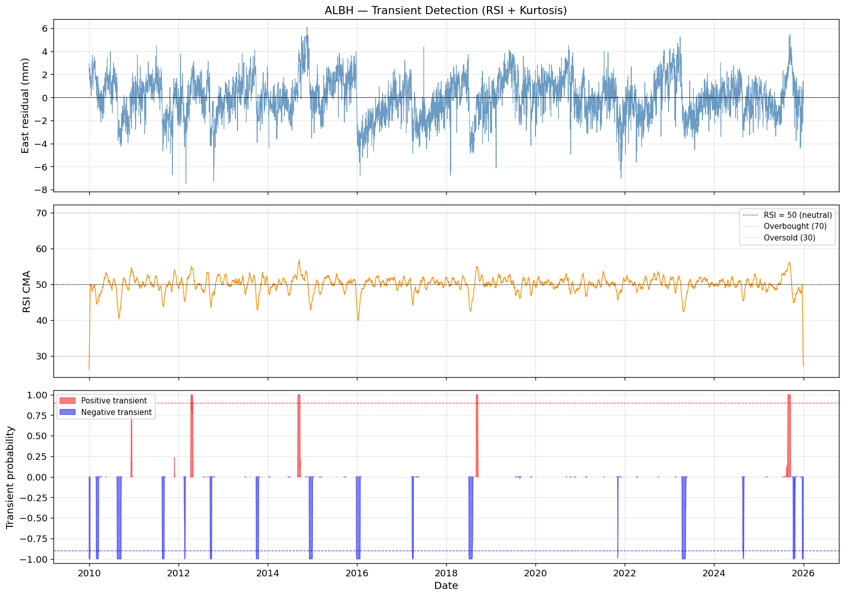
# ── Full probability time series plot ────────────────────────────────────
fig, axes = plt.subplots(3, 1, figsize=(14, 10), sharex=True)

# A. East residual displacement
axes[0].plot(df_albh.time, df_albh.east_res, 'steelblue', lw=0.7, alpha=0.8)
axes[0].axhline(0, color='k', lw=0.5)
axes[0].set_ylabel("East residual (mm)")
axes[0].set_title("ALBH — Transient Detection (RSI + Kurtosis)")
axes[0].grid(True, alpha=0.3)

# B. RSI CMA
axes[1].plot(df_albh.time, df_albh.east_cma, 'darkorange', lw=0.9)
axes[1].axhline(50, color='k', lw=0.5, ls='--', label='RSI = 50 (neutral)')
axes[1].axhline(70, color='red', lw=0.5, ls=':', alpha=0.7, label='Overbought (70)')
axes[1].axhline(30, color='green', lw=0.5, ls=':', alpha=0.7, label='Oversold (30)')
axes[1].set_ylabel("RSI CMA")
axes[1].legend(fontsize=9)
axes[1].grid(True, alpha=0.3)

# C. Kurtosis probability
axes[2].fill_between(df_albh.time, 0, df_albh.east_prob,
                     where=df_albh.east_prob > 0, color='red', alpha=0.5, label='Positive transient')
axes[2].fill_between(df_albh.time, 0, df_albh.east_prob,
                     where=df_albh.east_prob < 0, color='blue', alpha=0.5, label='Negative transient')
axes[2].axhline(0.9, color='red', lw=0.8, ls='--', alpha=0.7)
axes[2].axhline(-0.9, color='blue', lw=0.8, ls='--', alpha=0.7)
axes[2].set_ylabel("Transient probability")
axes[2].set_xlabel("Date")
axes[2].set_ylim(-1.05, 1.05)
axes[2].legend(fontsize=9)
axes[2].grid(True, alpha=0.3)

plt.tight_layout()
plt.show()
10. Identify Slow Slip Events#
From the probability time series, we extract the time periods of significant transient activity. These correspond to ETS events in Cascadia, which recur approximately every 12–14 months near ALBH.
# ── Identify transient windows ────────────────────────────────────────────
PROB_THRESHOLD = 0.85       # probability threshold for detection
MIN_DURATION   = 5        # minimum consecutive days above threshold

prob = df_albh.east_prob.values
time = df_albh.time.values

# Label positive transient days
pos_flag = np.absolute(prob) > PROB_THRESHOLD
# Cluster into events
from itertools import groupby

events = []
for key, group in groupby(enumerate(pos_flag), key=lambda x: x[1]):
    if key:
        indices = [i for i, _ in group]
        if len(indices) >= MIN_DURATION:
            t_start = pd.Timestamp(time[indices[0]])
            t_end   = pd.Timestamp(time[indices[-1]])
            peak_prob = prob[indices].max()
            peak_date = pd.Timestamp(time[indices[np.argmax(prob[indices])]])
            events.append({
                'start'    : t_start,
                'end'      : t_end,
                'peak_date': peak_date,
                'duration' : len(indices),
                'max_prob' : peak_prob,
            })

print(f"Detected {len(events)} positive transient events (prob > {PROB_THRESHOLD}, ≥{MIN_DURATION} days):")
print()
print(f"{'#':<4} {'Start':<12} {'End':<12} {'Peak':<12} {'Dur(days)':<12} {'Max prob':<10}")
print("-" * 60)
for i, ev in enumerate(events):
    print(f"{i:<4} {str(ev['start'].date()):<12} {str(ev['end'].date()):<12} "
          f"{str(ev['peak_date'].date()):<12} {ev['duration']:<12} {ev['max_prob']:.4f}")
Detected 21 positive transient events (prob > 0.85, ≥5 days):

#    Start        End          Peak         Dur(days)    Max prob
------------------------------------------------------------
0    2010-01-01   2010-01-09   2010-01-09   9            -0.9996
1    2010-03-01   2010-03-20   2010-03-19   20           -0.8888
2    2010-08-19   2010-09-20   2010-08-19   33           -0.9972
3    2010-12-12   2010-12-16   2010-12-15   5            1.0000
4    2011-08-23   2011-09-07   2011-08-23   16           -0.9753
5    2012-02-22   2012-02-26   2012-02-26   5            -0.9718
6    2012-04-13   2012-04-20   2012-04-19   8            1.0000
7    2012-04-24   2012-04-29   2012-04-26   6            0.9982
8    2012-09-18   2012-09-30   2012-09-18   13           -0.9852
9    2013-09-30   2013-10-18   2013-10-18   19           -0.9968
10   2014-09-05   2014-09-22   2014-09-08   18           1.0000
11   2014-12-08   2015-01-02   2015-01-02   26           -0.9783
12   2015-12-28   2016-01-27   2015-12-28   31           -0.9678
13   2017-03-29   2017-04-07   2017-03-29   10           -0.9088
14   2018-07-06   2018-08-03   2018-08-03   29           -0.8674
15   2018-09-04   2018-09-16   2018-09-10   13           1.0000
16   2023-04-15   2023-05-12   2023-05-12   28           -0.9391
17   2024-08-26   2024-08-31   2024-08-31   6            -0.9321
18   2025-08-27   2025-09-16   2025-08-28   21           1.0000
19   2025-10-09   2025-10-19   2025-10-19   11           -0.9578
20   2025-12-23   2025-12-31   2025-12-23   9            -0.9809
11. Extract and Analyze a Single Slow Slip Event#
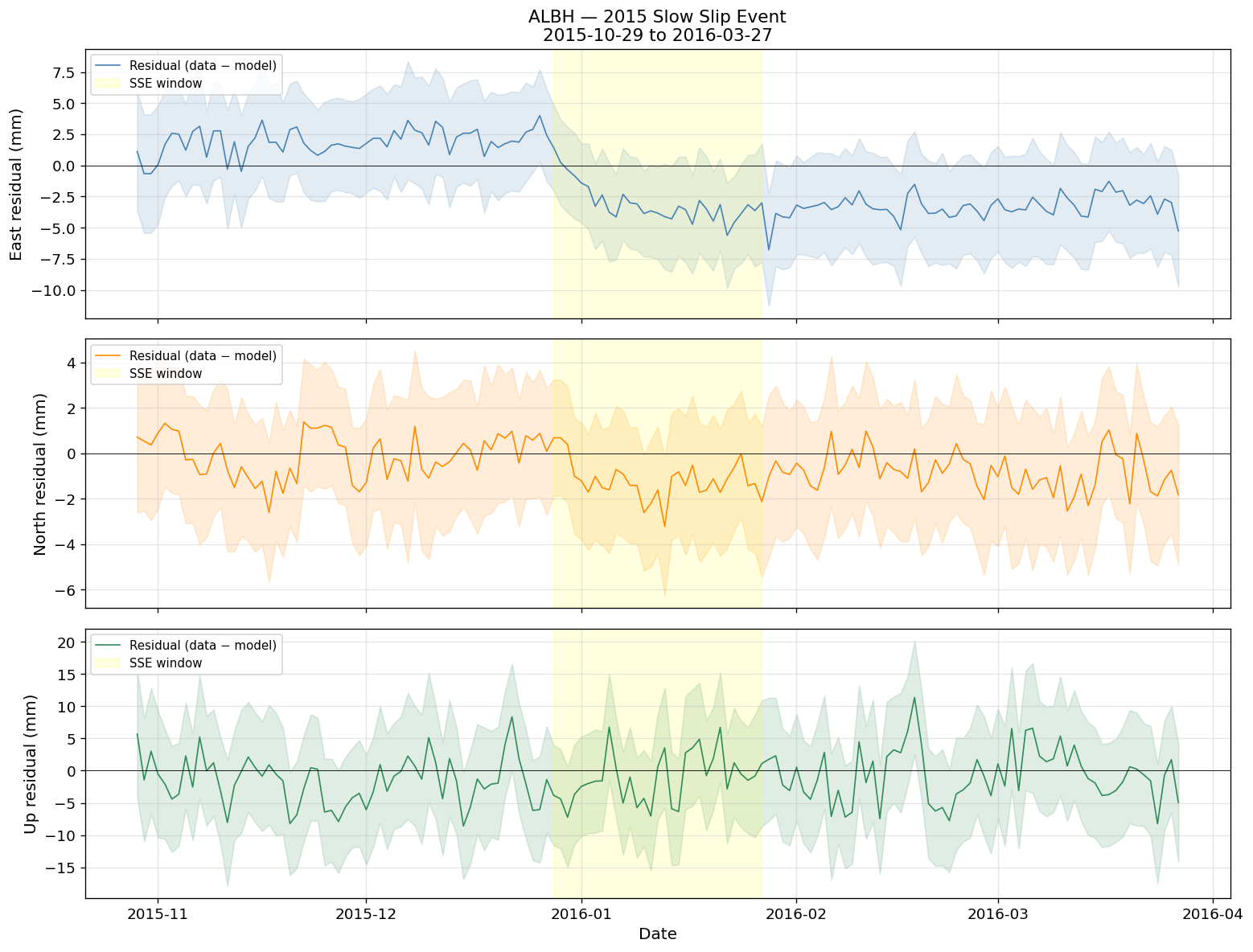
We now zoom into one well-defined slow slip event for detailed analysis. The late-2015 Cascadia ETS event (December 2015 to January 2016) is one of the strongest in the instrumental record near Victoria, BC and is clearly visible at ALBH.
We will:
Window the data around the event
Fit pre- and post-event linear trends
Estimate the coseismic-style offset
Characterize the temporal evolution (onset ramp)
# ── Select event for detailed analysis ────────────────────────────────────
# Change these dates to examine different events
SSE_TSTART = '2015-12-28'
SSE_TEND   = '2016-01-27'

# Pre-event reference window (60 days before start)
PRE_DAYS  = 60
POST_DAYS = 60

t_event_start = pd.Timestamp(SSE_TSTART)
t_event_end   = pd.Timestamp(SSE_TEND)
t_pre_start   = t_event_start - pd.Timedelta(days=PRE_DAYS)
t_post_end    = t_event_end   + pd.Timedelta(days=POST_DAYS)

# Subset the data
mask_event = (df_albh.time >= t_event_start) & (df_albh.time <= t_event_end)
mask_window = (df_albh.time >= t_pre_start)  & (df_albh.time <= t_post_end)

df_sse    = df_albh[mask_event].copy()
df_window = df_albh[mask_window].copy()

print(f"Event window   : {SSE_TSTART} → {SSE_TEND} ({mask_event.sum()} days)")
print(f"Analysis window: {t_pre_start.date()} → {t_post_end.date()} ({mask_window.sum()} days)")
print(f"\nPeak east residual during event: {df_sse.east_res.max():.2f} mm")
print(f"Peak north residual during event: {df_albh.loc[mask_event,'north_mm'].sub(results['north_mm']['fit'][mask_event]).max():.2f} mm")
Event window   : 2015-12-28 → 2016-01-27 (31 days)
Analysis window: 2015-10-29 → 2016-03-27 (151 days)

Peak east residual during event: 1.43 mm
Peak north residual during event: 0.69 mm
# ── 3-component zoom on the SSE ──────────────────────────────────────────
fig, axes = plt.subplots(3, 1, figsize=(13, 10), sharex=True)

comp_info_res = [
    ('east_mm',  'east_res',  'East',  'steelblue'),
    ('north_mm', None,        'North', 'darkorange'),
    ('up_mm',    None,        'Up',    'seagreen'),
]

for ax, (comp, res_key, label, color) in zip(axes, comp_info_res):
    r = results[comp]

    # Full signal in window
    sig = df_albh.loc[mask_window, comp].values
    res = (df_albh.loc[mask_window, comp].values - r['fit'][mask_window])
    t_win = df_albh.loc[mask_window, 'time'].values

    # Plot raw residual
    ax.plot(t_win, res, color=color, lw=1.0, label='Residual (data − model)')
    ax.fill_between(t_win, res - 2*df_albh.loc[mask_window, comp.replace('_mm','_sig')].values,
                    res + 2*df_albh.loc[mask_window, comp.replace('_mm','_sig')].values,
                    alpha=0.15, color=color)

    # Shade event period
    ax.axvspan(np.datetime64(SSE_TSTART), np.datetime64(SSE_TEND),
               alpha=0.12, color='yellow', label='SSE window')
    ax.axhline(0, color='k', lw=0.5)

    ax.set_ylabel(f"{label} residual (mm)")
    ax.legend(loc='upper left', fontsize=9)
    ax.grid(True, alpha=0.3)

axes[0].set_title("ALBH — 2015 Slow Slip Event\n" + str(t_pre_start.date()) + " to " + str(t_post_end.date()))
axes[2].set_xlabel("Date")
plt.tight_layout()
plt.show()
12. Offset Estimation for the Slow Slip Event#
We use two complementary methods to estimate the displacement offsets produced by the slow slip event:
Method 1: Pre/Post Mean Differencing#
Compute the mean residual displacement in a reference window before the event and subtract from the mean in a post-event window. This is robust but assumes linear behavior in the windows.
Method 2: Step Function Fit#
Add a Heaviside step at the event onset to the existing model and solve for the step amplitude via weighted least squares. This is more principled and produces formal uncertainties.
# ── Method 1: Pre/Post mean differencing ──────────────────────────────────

# Define reference windows
PRE_WIN_DAYS  = 14   # days before event start to average
POST_WIN_DAYS = 14   # days after event end to average

t_pre_end    = t_event_start - pd.Timedelta(days=5)   # small gap before event
t_pre_start2 = t_pre_end     - pd.Timedelta(days=PRE_WIN_DAYS)
t_post_start = t_event_end   + pd.Timedelta(days=5)   # small gap after event
t_post_end2  = t_post_start  + pd.Timedelta(days=POST_WIN_DAYS)

mask_pre  = (df_albh.time >= t_pre_start2) & (df_albh.time <= t_pre_end)
mask_post = (df_albh.time >= t_post_start) & (df_albh.time <= t_post_end2)

print("=" * 55)
print("Method 1: Pre/Post Mean Differencing")
print("=" * 55)
print(f"Pre-event  window: {t_pre_start2.date()} → {t_pre_end.date()} ({mask_pre.sum()} pts)")
print(f"Post-event window: {t_post_start.date()} → {t_post_end2.date()} ({mask_post.sum()} pts)")
print()

offsets_m1 = {}
for comp, label, color in comp_info:
    r = results[comp]
    res = df_albh[comp].values - r['fit']   # residuals
    sig = df_albh[comp.replace('_mm','_sig')].values

    pre_vals  = res[mask_pre];   pre_sig  = sig[mask_pre]
    post_vals = res[mask_post];  post_sig = sig[mask_post]

    # Weighted means
    w_pre   = 1/pre_sig**2;   mean_pre  = np.nansum(pre_vals  * w_pre)  / np.nansum(w_pre)
    w_post  = 1/post_sig**2;  mean_post = np.nansum(post_vals * w_post) / np.nansum(w_post)

    # Formal uncertainties on weighted means
    n_pre   = np.sum(~np.isnan(pre_vals))
    n_post  = np.sum(~np.isnan(post_vals))
    unc_pre  = 1/np.sqrt(np.nansum(w_pre))
    unc_post = 1/np.sqrt(np.nansum(w_post))

    offset = mean_post - mean_pre
    unc_offset = np.sqrt(unc_pre**2 + unc_post**2)

    offsets_m1[comp] = (offset, unc_offset)
    print(f"  {label:6s}: pre = {mean_pre:+.3f} mm  |  post = {mean_post:+.3f} mm  "
          f"|  Δ = {offset:+.3f} ± {unc_offset:.3f} mm")
=======================================================
Method 1: Pre/Post Mean Differencing
=======================================================
Pre-event  window: 2015-12-09 → 2015-12-23 (15 pts)
Post-event window: 2016-02-01 → 2016-02-15 (15 pts)

  East  : pre = +2.137 mm  |  post = -3.242 mm  |  Δ = -5.380 ± 0.753 mm
  North : pre = +0.006 mm  |  post = -0.478 mm  |  Δ = -0.484 ± 0.539 mm
  Up    : pre = -0.493 mm  |  post = -1.926 mm  |  Δ = -1.432 ± 1.578 mm
# ── Method 2: Step function least-squares fit ────────────────────────────
print("=" * 55)
print("Method 2: Step Function Least Squares")
print("=" * 55)
print()

# Add a step at the event onset
SSE_EPOCH = float(pd.Timestamp(SSE_TSTART).year +
                  (pd.Timestamp(SSE_TSTART) - pd.Timestamp(f'{pd.Timestamp(SSE_TSTART).year}-01-01')).days
                  / (366 if pd.Timestamp(SSE_TSTART).is_leap_year else 365))

# Also include original coseismic epochs
all_steps = unique_epochs + [SSE_EPOCH]

offsets_m2 = {}
for comp, label, color in comp_info:
    sig_col = comp.replace('_mm','_sig')
    r_new = fit_model(
        dec_year, df_albh[comp].values,
        sigma_mm=df_albh[sig_col].values,
        coseismic_times=all_steps
    )
    # SSE step is the LAST column
    sse_idx  = len(r_new['params']) - 1
    offset   = r_new['params'][sse_idx]
    unc      = r_new['param_std'][sse_idx]
    offsets_m2[comp] = (offset, unc)
    print(f"  {label:6s}: SSE offset = {offset:+.3f} ± {unc:.3f} mm")
=======================================================
Method 2: Step Function Least Squares
=======================================================

  East  : SSE offset = -2.749 ± 0.142 mm
  North : SSE offset = -0.189 ± 0.101 mm
  Up    : SSE offset = -1.400 ± 0.303 mm
# ── Compare methods ──────────────────────────────────────────────────────
print("\n" + "=" * 55)
print("Comparison of offset estimates")
print("=" * 55)
print(f"{'Component':<10} {'Method1 (mm)':<20} {'Method2 (mm)':<20} {'Agree?'}")
print("-" * 60)
for comp, label, _ in comp_info:
    o1, u1 = offsets_m1[comp]
    o2, u2 = offsets_m2[comp]
    # 2-sigma agreement
    agree = abs(o1 - o2) < 2*np.sqrt(u1**2 + u2**2)
    print(f"{label:<10} {o1:+.3f} ± {u1:.3f}      {o2:+.3f} ± {u2:.3f}      {'✓' if agree else '✗'}")
=======================================================
Comparison of offset estimates
=======================================================
Component  Method1 (mm)         Method2 (mm)         Agree?
------------------------------------------------------------
East       -5.380 ± 0.753      -2.749 ± 0.142      ✗
North      -0.484 ± 0.539      -0.189 ± 0.101      ✓
Up         -1.432 ± 1.578      -1.400 ± 0.303      ✓
13. Temporal Evolution of the Slow Slip Event#
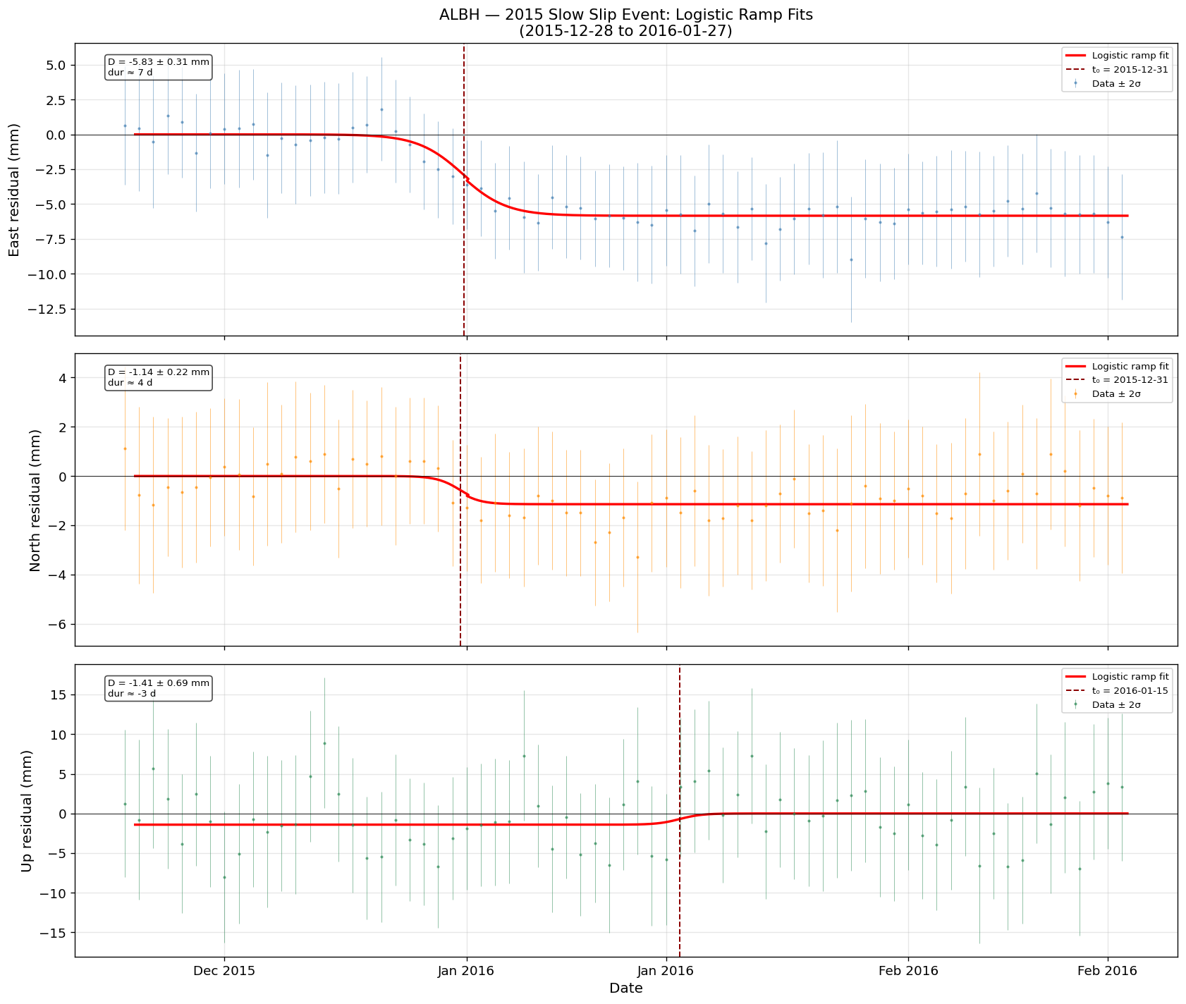
Beyond the total offset, the temporal evolution of the slow slip constrains the rupture process. We fit a logistic (sigmoid) function to model the displacement ramp:
where \(D\) is the total offset, \(k\) is the rise rate, and \(t_0\) is the inflection point (approximate event midpoint).
def logistic_ramp(t, D, k, t0):
    return D / (1 + np.exp(-k * (t - t0)))

# ── Fit logistic ramp to all 3 components ────────────────────────────────
mask_broad = ((df_albh.time >= t_event_start - pd.Timedelta(days=20)) &
              (df_albh.time <= t_event_end   + pd.Timedelta(days=20)))

fit_results = {}
comp_info_fit = [
    ('east_mm',  'east_sig',  'East'),
    ('north_mm', 'north_sig', 'North'),
    ('up_mm',    'up_sig',    'Up'),
]

for comp, sig_comp, label in comp_info_fit:
    t_fit = df_albh.loc[mask_broad, 'dec_year'].values
    d_fit = (df_albh.loc[mask_broad, comp].values -
             results[comp]['fit'][mask_broad])
    s_fit = df_albh.loc[mask_broad, sig_comp].values

    ok = ~np.isnan(d_fit) & ~np.isnan(s_fit)
    t_f, d_f, s_f = t_fit[ok], d_fit[ok], s_fit[ok]

    baseline = np.nanmean(d_f[:15])
    d_f_centered = d_f - baseline

    try:
        D0  = d_f_centered.max() - d_f_centered.min()
        t00 = (t_f[0] + t_f[-1]) / 2
        popt, pcov = curve_fit(logistic_ramp, t_f, d_f_centered,
                               p0=[D0, 30, t00], maxfev=10000,
                               sigma=s_f, absolute_sigma=True)
        perr = np.sqrt(np.diag(pcov))
        D_fit, k_fit, t0_fit = popt
        D_err, k_err, t0_err = perr
        t0_approx = (pd.Timestamp(f'{int(t0_fit)}-01-01')
                     + pd.Timedelta(days=(t0_fit % 1)*365.25))
        duration_days = 2 * np.log(9) / k_fit * 365.25

        fit_results[comp] = {
            'popt'         : popt,
            'perr'         : perr,
            'D'            : D_fit,   'D_err' : D_err,
            'k'            : k_fit,   'k_err' : k_err,
            't0'           : t0_fit,  't0_err': t0_err,
            't0_date'      : t0_approx,
            'duration_days': duration_days,
            'baseline'     : baseline,
            'success'      : True,
        }
        print(f"{label} component:")
        print(f"  Total offset D = {D_fit:+.3f} ± {D_err:.3f} mm")
        print(f"  Rise rate k    = {k_fit:.2f}  ± {k_err:.2f} yr⁻¹")
        print(f"  Midpoint t₀    = {t0_approx.date()}")
        print(f"  10–90% duration≈ {duration_days:.1f} days")
        print()

    except Exception as e:
        fit_results[comp] = {'success': False}
        print(f"{label} component: fit failed — {e}\n")
East component:
  Total offset D = -5.834 ± 0.313 mm
  Rise rate k    = 226.35  ± 118.69 yr⁻¹
  Midpoint t₀    = 2015-12-31
  10–90% duration≈ 7.1 days

North component:
  Total offset D = -1.143 ± 0.216 mm
  Rise rate k    = 444.99  ± 1205.99 yr⁻¹
  Midpoint t₀    = 2015-12-31
  10–90% duration≈ 3.6 days

Up component:
  Total offset D = -1.414 ± 0.689 mm
  Rise rate k    = -467.92  ± 3592.96 yr⁻¹
  Midpoint t₀    = 2016-01-15
  10–90% duration≈ -3.4 days
fig, axes = plt.subplots(3, 1, figsize=(14, 12), sharex=True)

comp_info_plot = [
    ('east_mm',  'east_sig',  'East',  'steelblue'),
    ('north_mm', 'north_sig', 'North', 'darkorange'),
    ('up_mm',    'up_sig',    'Up',    'seagreen'),
]

t_day = df_albh.loc[mask_broad, 'time'].values
t_yr  = df_albh.loc[mask_broad, 'dec_year'].values

for ax, (comp, sig_comp, label, color) in zip(axes, comp_info_plot):
    d_res = (df_albh.loc[mask_broad, comp].values -
             results[comp]['fit'][mask_broad])
    s_res = df_albh.loc[mask_broad, sig_comp].values
    baseline = (fit_results[comp]['baseline'] if fit_results[comp]['success']
                else np.nanmean(d_res[:15]))
    d_centered = d_res - baseline

    ax.errorbar(t_day, d_centered, yerr=2*s_res, fmt='.',
                color=color, ms=3, elinewidth=0.5, alpha=0.6, label='Data ± 2σ')

    if fit_results[comp]['success']:
        popt = fit_results[comp]['popt']
        t_fine = np.linspace(t_yr[~np.isnan(t_yr)].min(),
                             t_yr[~np.isnan(t_yr)].max(), 500)
        d_model = logistic_ramp(t_fine, *popt)
        t_fine_dt = [pd.Timestamp(f'{int(tt)}-01-01')
                     + pd.Timedelta(days=(tt % 1)*365.25) for tt in t_fine]
        ax.plot(t_fine_dt, d_model, 'r-', lw=2, label='Logistic ramp fit')
        ax.axvline(fit_results[comp]['t0_date'], color='darkred', ls='--', lw=1.2,
                   label=f"t₀ = {fit_results[comp]['t0_date'].date()}")
        ax.text(0.03, 0.95,
                f"D = {fit_results[comp]['D']:+.2f} ± {fit_results[comp]['D_err']:.2f} mm\n"
                f"dur ≈ {fit_results[comp]['duration_days']:.0f} d",
                transform=ax.transAxes, fontsize=8, va='top',
                bbox=dict(boxstyle='round,pad=0.3', fc='white', alpha=0.7))

    ax.axhline(0, color='k', lw=0.5)
    ax.set_ylabel(f"{label} residual (mm)")
    ax.legend(fontsize=8)
    ax.grid(True, alpha=0.3)

axes[0].set_title("ALBH — 2015 Slow Slip Event: Logistic Ramp Fits\n"
                  f"({SSE_TSTART} to {SSE_TEND})")
axes[-1].set_xlabel("Date")
axes[-1].xaxis.set_major_formatter(mdates.DateFormatter('%b %Y'))
plt.tight_layout()
plt.show()
14. Displacement Vector and Interpretation#
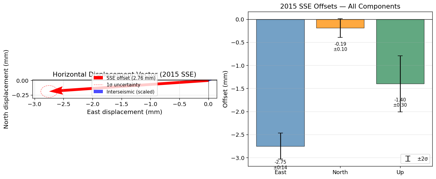
The horizontal displacement vector (East, North offset) during slow slip should point roughly trench-ward (southwest at ALBH), opposite to the long-term interseismic direction. This is a key diagnostic for ETS events.
# ── Compile offset table ─────────────────────────────────────────────────
print("=" * 60)
print("2015 SSE Offset Summary — Station ALBH")
print("=" * 60)
print()

offsets = {
    'East (mm)' : offsets_m2['east_mm'],
    'North (mm)': offsets_m2['north_mm'],
    'Up (mm)'   : offsets_m2['up_mm'],
}

for name, (val, unc) in offsets.items():
    snr = abs(val) / unc if unc > 0 else 0
    sig_str = f"{snr:.1f}σ" if snr >= 1 else "<1σ"
    print(f"  {name:<12}: {val:+.3f} ± {unc:.3f} mm  ({sig_str})")

# Horizontal magnitude
E_off, E_unc = offsets_m2['east_mm']
N_off, N_unc = offsets_m2['north_mm']
H_mag = np.sqrt(E_off**2 + N_off**2)
H_unc = np.sqrt((E_off*E_unc)**2 + (N_off*N_unc)**2) / H_mag

# Azimuth of horizontal vector
azimuth = np.degrees(np.arctan2(E_off, N_off)) % 360

print()
print(f"  Horizontal magnitude: {H_mag:.3f} ± {H_unc:.3f} mm")
print(f"  Horizontal azimuth  : {azimuth:.1f}°")
print()
print("Note: Cascadia ETS offsets at ALBH typically trend ~240° (SW), opposite")
print("to the ~060° interseismic direction — toward the locked interface.")
============================================================
2015 SSE Offset Summary — Station ALBH
============================================================

  East (mm)   : -2.749 ± 0.142 mm  (19.3σ)
  North (mm)  : -0.189 ± 0.101 mm  (1.9σ)
  Up (mm)     : -1.400 ± 0.303 mm  (4.6σ)

  Horizontal magnitude: 2.756 ± 0.142 mm
  Horizontal azimuth  : 266.1°

Note: Cascadia ETS offsets at ALBH typically trend ~240° (SW), opposite
to the ~060° interseismic direction — toward the locked interface.
# ── Displacement vector plot ─────────────────────────────────────────────
fig, axes = plt.subplots(1, 2, figsize=(12, 5))

# Left: map view of offset vector
ax = axes[0]
ax.quiver(0, 0, E_off, N_off,
          angles='xy', scale_units='xy', scale=1,
          color='red', width=0.015, label=f'SSE offset ({H_mag:.2f} mm)')

# Add uncertainty ellipse (assumes uncorrelated)
theta = np.linspace(0, 2*np.pi, 100)
ax.plot(E_off + E_unc*np.cos(theta), N_off + N_unc*np.sin(theta),
        'r--', lw=0.8, alpha=0.6, label='1σ uncertainty')

# Interseismic velocity direction (approximate for ALBH ~ 60° azimuth)
v_e = 3.0; v_n = 1.5   # mm/yr approximate
ax.quiver(0, 0, v_e, v_n,
          angles='xy', scale_units='xy', scale=1,
          color='blue', width=0.012, alpha=0.7, label=f'Interseismic (scaled)')

ax.axhline(0, color='k', lw=0.5); ax.axvline(0, color='k', lw=0.5)
ax.set_xlabel("East displacement (mm)")
ax.set_ylabel("North displacement (mm)")
ax.set_title("Horizontal Displacement Vector (2015 SSE)")
ax.legend(fontsize=9)
ax.set_aspect('equal')
ax.grid(True, alpha=0.3)

# Right: 3-component bar chart
ax2 = axes[1]
components = ['East', 'North', 'Up']
vals  = [offsets_m2['east_mm'][0], offsets_m2['north_mm'][0], offsets_m2['up_mm'][0]]
uncs  = [offsets_m2['east_mm'][1], offsets_m2['north_mm'][1], offsets_m2['up_mm'][1]]
colors = ['steelblue', 'darkorange', 'seagreen']

bars = ax2.bar(components, vals, color=colors, alpha=0.75, edgecolor='k', linewidth=0.8)
ax2.errorbar(components, vals, yerr=2*np.array(uncs), fmt='none',
             color='black', capsize=5, lw=1.5, label='±2σ')
ax2.axhline(0, color='k', lw=0.8)
ax2.set_ylabel("Offset (mm)")
ax2.set_title("2015 SSE Offsets — All Components")
ax2.legend()
ax2.grid(True, alpha=0.3, axis='y')

# Annotate bars
for bar, val, unc in zip(bars, vals, uncs):
    ax2.text(bar.get_x() + bar.get_width()/2, val + 0.15 if val > 0 else val - 0.3,
             f'{val:+.2f}\n±{unc:.2f}', ha='center', va='bottom' if val > 0 else 'top',
             fontsize=9)

plt.tight_layout()
plt.show()
15. Multi-Station Analysis#
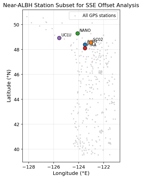
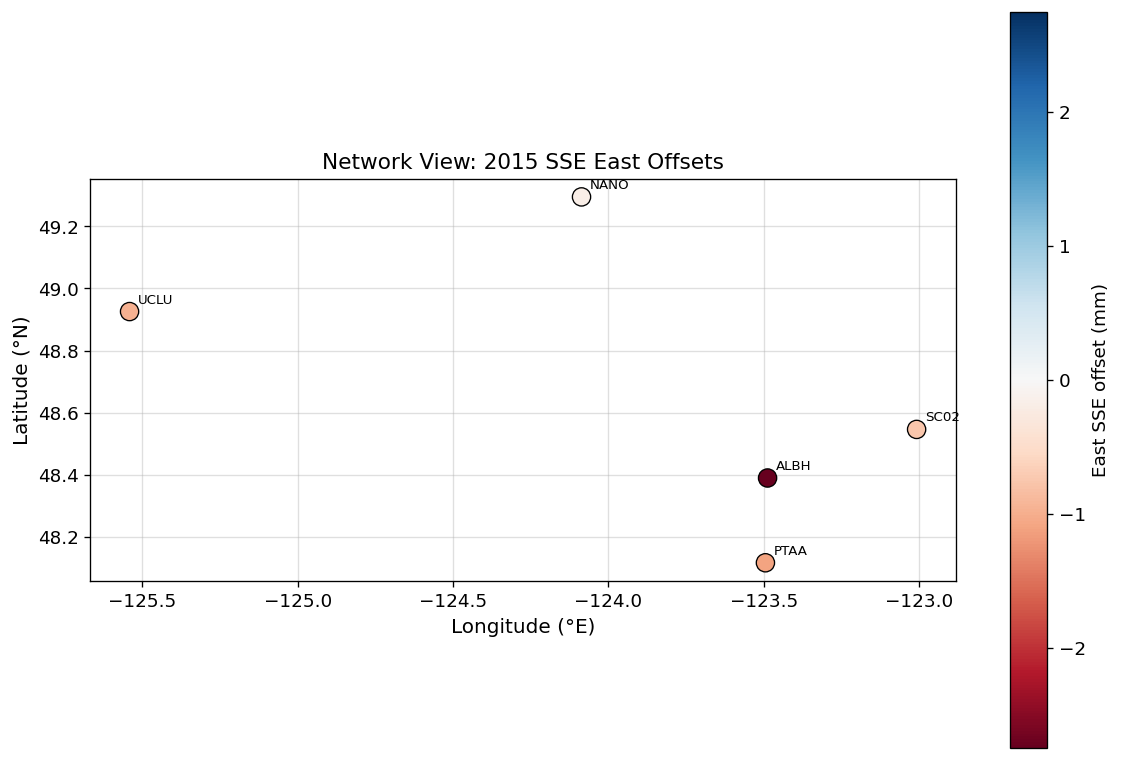
Slow slip events coherently displace a network of stations. We examine a small subset of stations closely surrounding ALBH to validate the SSE detection spatially and to compare offset magnitudes across the near-field network.
We restrict the analysis to a compact cluster within ~200 km of ALBH (southern Vancouver Island / northern Puget Sound), avoiding distant stations where the ETS signal is weaker and the step-function SSE model becomes less appropriate.
# ── Select a small subset of stations near ALBH ─────────────────────────────
# Restricting to the compact cluster on southern Vancouver Island / northern
# Washington that sits directly above the ETS source region near ALBH.
# These stations are all within ~150 km of ALBH and have long records.
albh_subset = ['albh', 'sc02', 'drao', 'nano', 'pnra', 'ptaa', 'uclu']

available = [s for s in albh_subset
             if s in ds.station.values and
             not np.all(np.isnan(ds.sel(station=s).east_m.values))]
print(f"Stations in near-ALBH subset: {available}")

# Quick map to confirm geographic clustering
fig, ax = plt.subplots(figsize=(8, 6))
ax.scatter(ds_plot.lon, ds_plot.lat, s=4, c='lightgray', zorder=2, label='All GPS stations')
for sname in available:
    sv = ds.sel(station=sname)
    ax.scatter(float(sv.lon), float(sv.lat), s=80, zorder=5, edgecolors='k', linewidths=0.7)
    ax.annotate(sname.upper(), (float(sv.lon), float(sv.lat)),
                xytext=(5, 4), textcoords='offset points', fontsize=9)
ax.set_xlabel("Longitude (°E)"); ax.set_ylabel("Latitude (°N)")
ax.set_title("Near-ALBH Station Subset for SSE Offset Analysis")
ax.legend(); ax.grid(True, alpha=0.3)
ax.set_aspect('equal', adjustable='box')
plt.tight_layout(); plt.show()
Stations in near-ALBH subset: ['albh', 'sc02', 'nano', 'ptaa', 'uclu']
# ── Compute SSE offsets for the near-ALBH subset ────────────────────────────
print("Computing SSE offsets for near-ALBH subset...")

network_results = {}
for sname in available:
    stat_i = ds.sel(station=sname)
    dec_yr_i = stat_i.dec_year.values
    east_i   = stat_i.east_m.values  * 1000
    esig_i   = stat_i.east_sigma_m.values * 1000

    try:
        r_i = fit_model(dec_yr_i, east_i, sigma_mm=esig_i,
                        coseismic_times=all_steps)
        east_off = r_i['params'][-1]
        east_unc = r_i['param_std'][-1]
        lat_i = float(stat_i.lat)
        lon_i = float(stat_i.lon)
        network_results[sname] = {
            'lat': lat_i, 'lon': lon_i,
            'east_off': east_off, 'east_unc': east_unc,
        }
        print(f"  {sname.upper():6s}  lat={lat_i:.2f}  lon={lon_i:.2f}  "
              f"E_off = {east_off:+.2f} ± {east_unc:.2f} mm")
    except Exception as e:
        print(f"  {sname.upper():6s}  FAILED: {e}")

print(f"\nCompleted {len(network_results)} stations.")
Computing SSE offsets for near-ALBH subset...
  ALBH    lat=48.39  lon=-123.49  E_off = -2.75 ± 0.14 mm
  SC02    lat=48.55  lon=-123.01  E_off = -0.76 ± 0.17 mm
  NANO    lat=49.29  lon=-124.09  E_off = -0.19 ± 0.12 mm
  PTAA    lat=48.12  lon=-123.49  E_off = -1.11 ± 0.16 mm
  UCLU    lat=48.93  lon=-125.54  E_off = -0.98 ± 0.14 mm

Completed 5 stations.
# ── Map of SSE offsets across the network ─────────────────────────────────
if len(network_results) >= 2:
    fig, ax = plt.subplots(figsize=(10, 8))

    lats = [v['lat'] for v in network_results.values()]
    lons = [v['lon'] for v in network_results.values()]
    e_offs = np.array([v['east_off'] for v in network_results.values()])
    e_uncs = np.array([v['east_unc'] for v in network_results.values()])

    # Color by offset sign/magnitude
    vmax = max(abs(e_offs.min()), abs(e_offs.max()), 2)
    sc = ax.scatter(lons, lats, c=e_offs, cmap='RdBu', vmin=-vmax, vmax=vmax,
                    s=120, edgecolors='k', linewidths=0.8, zorder=5)

    # Annotate stations
    for sname, v in network_results.items():
        ax.annotate(sname.upper(), (v['lon'], v['lat']),
                    xytext=(5, 5), textcoords='offset points', fontsize=8)

    cbar = fig.colorbar(sc, ax=ax, shrink=0.8)
    cbar.set_label("East SSE offset (mm)", fontsize=11)
    ax.set_xlabel("Longitude (°E)")
    ax.set_ylabel("Latitude (°N)")
    ax.set_title("Network View: 2015 SSE East Offsets")
    ax.grid(True, alpha=0.4)
    ax.set_aspect('equal', adjustable='box')
    plt.tight_layout()
    plt.show()
else:
    print("Need at least 2 stations for network map.")
15e. Basic Time Series Analysis: SC02 and a Mendocino Triple Junction Station#
To extend our regional perspective, we perform the same basic signal decomposition workflow on two additional stations:
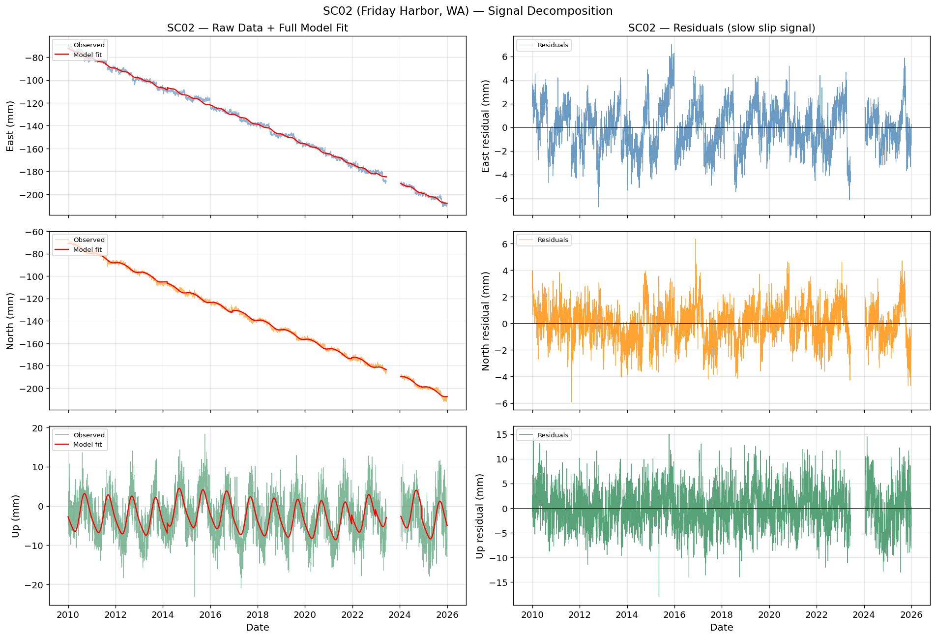
SC02 (Friday Harbor, San Juan Islands, WA) — a well-characterized continuous GPS site in the central Puget Sound, south of ALBH.
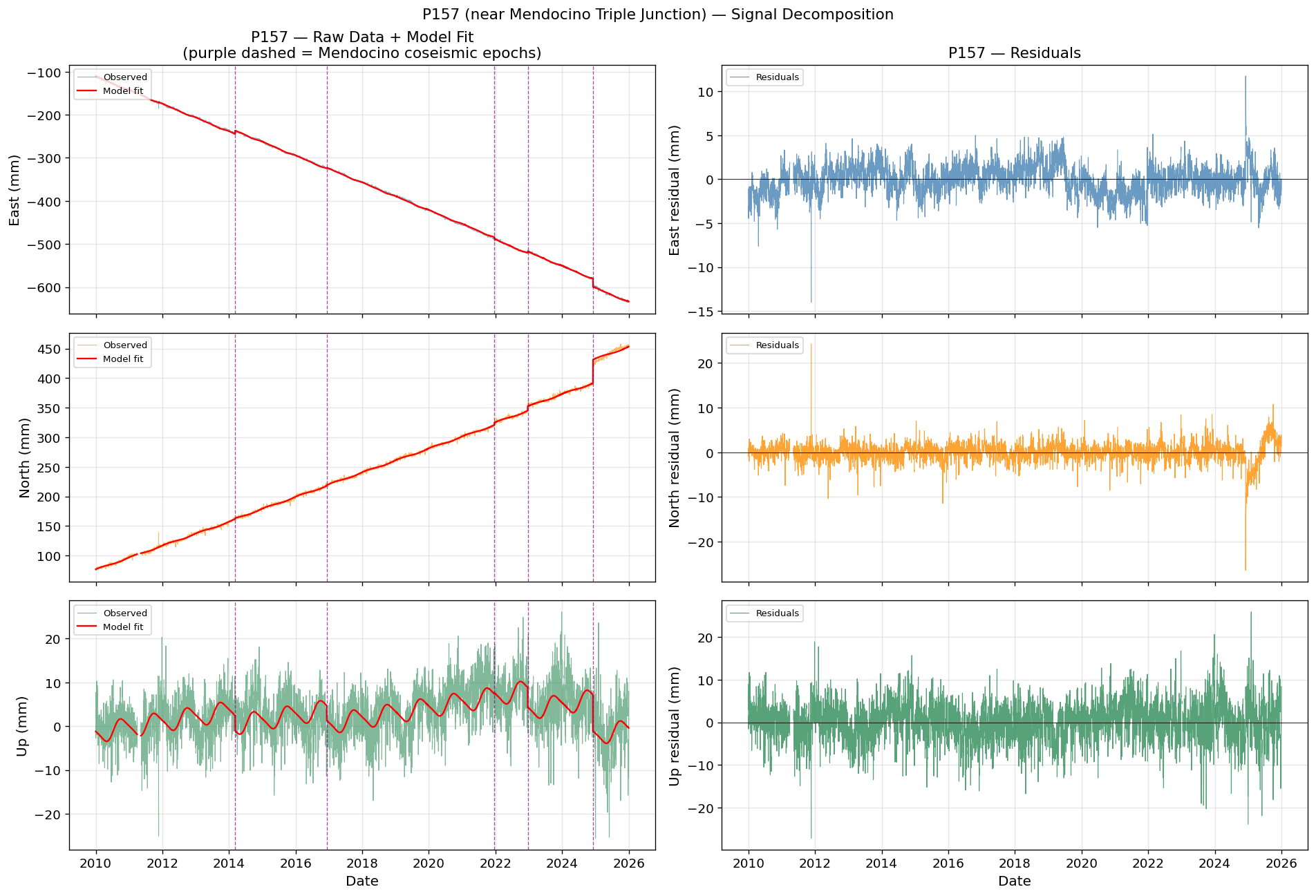
Mendocino station (near the Mendocino Triple Junction, ~40°N northern California) — the station closest to the coseismic sources in our catalog. Because it sits directly above or adjacent to the Mendocino Transform Fault and the Gorda slab, it experiences measurable static offsets from the M≥6 events and clear postseismic deformation.
We apply the same decomposition model (interseismic + seasonal + coseismic steps) to both stations, inspect the residuals, and set up the coseismic and postseismic analysis below.
# ── Load SC02 ────────────────────────────────────────────────────────────────
sc02_name = 'sc02'
if sc02_name not in ds.station.values:
    print(f"WARNING: {sc02_name} not found in dataset — check station name spelling.")
else:
    stat_sc02 = ds.sel(station=sc02_name)
    df_sc02 = pd.DataFrame({
        'time'      : pd.to_datetime(stat_sc02.time.values),
        'dec_year'  : stat_sc02.dec_year.values,
        'east_mm'   : stat_sc02.east_m.values  * 1000,
        'north_mm'  : stat_sc02.north_m.values * 1000,
        'up_mm'     : stat_sc02.up_m.values    * 1000,
        'east_sig'  : stat_sc02.east_sigma_m.values  * 1000,
        'north_sig' : stat_sc02.north_sigma_m.values * 1000,
        'up_sig'    : stat_sc02.up_sigma_m.values    * 1000,
    })
    print(f"Station SC02 — {df_sc02.shape[0]} daily observations")
    print(f"Date range   : {df_sc02.time.min().date()} → {df_sc02.time.max().date()}")
    for col in ['east_mm','north_mm','up_mm']:
        n_valid = df_sc02[col].notna().sum()
        print(f"  {col:12s}: {n_valid:5d} valid ({100*n_valid/len(df_sc02):.1f}%)")

    # Fit decomposition model to SC02
    dec_yr_sc02 = df_sc02.dec_year.values
    results_sc02 = {}
    for comp, label in [('east_mm','East'), ('north_mm','North'), ('up_mm','Up')]:
        sig_col = comp.replace('_mm','_sig')
        results_sc02[comp] = fit_model(
            dec_yr_sc02,
            df_sc02[comp].values,
            sigma_mm=df_sc02[sig_col].values,
            coseismic_times=unique_epochs   # NOTE: Mendocino quakes are far from SC02;
                                             # steps may be very small but we include them
                                             # for model consistency
        )
    print("\nSC02 — Fitted velocities:")
    for comp, label in [('east_mm','East'), ('north_mm','North'), ('up_mm','Up')]:
        vel = results_sc02[comp]['params'][1]
        vel_sig = results_sc02[comp]['param_std'][1]
        print(f"  {label}: {vel:+.3f} ± {vel_sig:.3f} mm/yr")
Station SC02 — 5844 daily observations
Date range   : 2010-01-01 → 2025-12-31
  east_mm     :  5620 valid (96.2%)
  north_mm    :  5620 valid (96.2%)
  up_mm       :  5620 valid (96.2%)

SC02 — Fitted velocities:
  East: -8.610 ± 0.031 mm/yr
  North: -8.528 ± 0.019 mm/yr
  Up: -0.328 ± 0.051 mm/yr
# ── SC02 decomposition plot ──────────────────────────────────────────────────
if 'df_sc02' in dir():
    fig, axes = plt.subplots(3, 2, figsize=(16, 11), sharex=True)
    comp_info_sc02 = [
        ('east_mm',  'East',  'steelblue'),
        ('north_mm', 'North', 'darkorange'),
        ('up_mm',    'Up',    'seagreen'),
    ]
    t_sc02 = df_sc02.time

    for row, (comp, label, color) in enumerate(comp_info_sc02):
        r = results_sc02[comp]

        # Left: raw + fit
        axes[row, 0].plot(t_sc02, df_sc02[comp], color=color, lw=0.7, alpha=0.6, label='Observed')
        axes[row, 0].plot(t_sc02, r['fit'], 'r-', lw=1.4, label='Model fit')
        axes[row, 0].set_ylabel(f"{label} (mm)")
        if row == 0:
            axes[row, 0].set_title("SC02 — Raw Data + Full Model Fit")
        axes[row, 0].legend(loc='upper left', fontsize=8)
        axes[row, 0].grid(True, alpha=0.3)

        # Right: residuals
        axes[row, 1].plot(t_sc02, r['residuals'], color=color, lw=0.7, alpha=0.8,
                          label='Residuals')
        axes[row, 1].axhline(0, color='k', lw=0.5)
        axes[row, 1].set_ylabel(f"{label} residual (mm)")
        if row == 0:
            axes[row, 1].set_title("SC02 — Residuals (slow slip signal)")
        axes[row, 1].legend(loc='upper left', fontsize=8)
        axes[row, 1].grid(True, alpha=0.3)

    for ax in axes[-1]:
        ax.set_xlabel("Date")

    plt.suptitle("SC02 (Friday Harbor, WA) — Signal Decomposition", fontsize=14)
    plt.tight_layout()
    plt.show()
# ── Select and load the nearest station to the Mendocino Triple Junction ────
# Candidate stations near ~40°N, ~124°W (Mendocino Triple Junction area).
# We search the dataset for the station with valid coordinates closest to
# the triple junction location.
MTJ_LAT = 40.30
MTJ_LON = -124.4

mendo_candidates = []
for sname in ds.station.values:
    lat_s = float(ds.sel(station=sname).lat)
    lon_s = float(ds.sel(station=sname).lon)
    if np.isnan(lat_s) or np.isnan(lon_s):
        continue
    # Filter to northern CA / extreme southern OR bounding box
    if 39.0 <= lat_s <= 42.5 and -126.0 <= lon_s <= -122.0:
        # Require reasonable data availability
        n_valid = np.sum(~np.isnan(ds.sel(station=sname).east_m.values))
        if n_valid > 365:
            dist = np.sqrt(((lat_s - MTJ_LAT)*111)**2 + ((lon_s - MTJ_LON)*111*np.cos(np.radians(MTJ_LAT)))**2)
            mendo_candidates.append((sname, lat_s, lon_s, dist, n_valid))

mendo_candidates.sort(key=lambda x: x[3])
print("Nearest stations to the Mendocino Triple Junction (sorted by distance):")
print(f"{'Station':<8} {'Lat':>7} {'Lon':>9} {'Dist(km)':>10} {'N_valid':>8}")
print("-" * 48)
for sname, lat_s, lon_s, dist, nv in mendo_candidates[:10]:
    print(f"{sname:<8} {lat_s:7.3f} {lon_s:9.3f} {dist:10.1f} {nv:8d}")

if mendo_candidates:
    MENDO_STATION = mendo_candidates[0][0]
    print(f"\nSelected Mendocino station: {MENDO_STATION.upper()}")
else:
    print("WARNING: No suitable station found near the Mendocino Triple Junction!")
    MENDO_STATION = None
Nearest stations to the Mendocino Triple Junction (sorted by distance):
Station      Lat       Lon   Dist(km)  N_valid
------------------------------------------------
p157      40.248  -124.308        9.7     5722
cme6      40.441  -124.396       15.7     3294
cme5      40.442  -124.396       15.7     3256
p159      40.505  -124.283       24.8     5577
p158      40.422  -124.107       28.3     5745
p163      40.220  -124.057       30.4     5833
p160      40.551  -124.133       35.9     5798
p161      40.637  -124.213       40.7     5807
p162      40.691  -124.237       45.6     5669
p165      40.246  -123.853       46.7     5781

Selected Mendocino station: P157
# ── Load the Mendocino station ───────────────────────────────────────────────
if MENDO_STATION is not None:
    stat_mendo = ds.sel(station=MENDO_STATION)
    df_mendo = pd.DataFrame({
        'time'      : pd.to_datetime(stat_mendo.time.values),
        'dec_year'  : stat_mendo.dec_year.values,
        'east_mm'   : stat_mendo.east_m.values  * 1000,
        'north_mm'  : stat_mendo.north_m.values * 1000,
        'up_mm'     : stat_mendo.up_m.values    * 1000,
        'east_sig'  : stat_mendo.east_sigma_m.values  * 1000,
        'north_sig' : stat_mendo.north_sigma_m.values * 1000,
        'up_sig'    : stat_mendo.up_sigma_m.values    * 1000,
    })
    mendo_lat = float(stat_mendo.lat)
    mendo_lon = float(stat_mendo.lon)
    print(f"Station {MENDO_STATION.upper()} ({mendo_lat:.3f}°N, {mendo_lon:.3f}°E)")
    print(f"Date range   : {df_mendo.time.min().date()} → {df_mendo.time.max().date()}")
    for col in ['east_mm','north_mm','up_mm']:
        n_valid = df_mendo[col].notna().sum()
        print(f"  {col:12s}: {n_valid:5d} valid ({100*n_valid/len(df_mendo):.1f}%)")

    # Fit decomposition model — include all Mendocino coseismic epochs
    dec_yr_mendo = df_mendo.dec_year.values
    results_mendo = {}
    for comp, label in [('east_mm','East'), ('north_mm','North'), ('up_mm','Up')]:
        sig_col = comp.replace('_mm','_sig')
        results_mendo[comp] = fit_model(
            dec_yr_mendo,
            df_mendo[comp].values,
            sigma_mm=df_mendo[sig_col].values,
            coseismic_times=unique_epochs
        )
    print("\nMendocino station — Fitted velocities (mm/yr):")
    for comp, label in [('east_mm','East'), ('north_mm','North'), ('up_mm','Up')]:
        vel = results_mendo[comp]['params'][1]
        vel_sig = results_mendo[comp]['param_std'][1]
        print(f"  {label}: {vel:+.3f} ± {vel_sig:.3f} mm/yr")
Station P157 (40.248°N, -124.308°E)
Date range   : 2010-01-01 → 2025-12-31
  east_mm     :  5722 valid (97.9%)
  north_mm    :  5722 valid (97.9%)
  up_mm       :  5722 valid (97.9%)

Mendocino station — Fitted velocities (mm/yr):
  East: -32.042 ± 0.021 mm/yr
  North: +20.213 ± 0.021 mm/yr
  Up: +1.255 ± 0.053 mm/yr
# ── Mendocino station decomposition plot ────────────────────────────────────
if MENDO_STATION is not None:
    fig, axes = plt.subplots(3, 2, figsize=(16, 11), sharex=True)
    t_mendo = df_mendo.time
    comp_info_mendo = [
        ('east_mm',  'East',  'steelblue'),
        ('north_mm', 'North', 'darkorange'),
        ('up_mm',    'Up',    'seagreen'),
    ]

    for row, (comp, label, color) in enumerate(comp_info_mendo):
        r = results_mendo[comp]

        # Left: raw + fit, mark coseismic epochs
        axes[row, 0].plot(t_mendo, df_mendo[comp], color=color, lw=0.7, alpha=0.6,
                          label='Observed')
        axes[row, 0].plot(t_mendo, r['fit'], 'r-', lw=1.4, label='Model fit')
        for t_co in unique_epochs:
            dt_co = pd.Timestamp(f'{int(t_co)}-01-01') + pd.Timedelta(days=(t_co % 1)*365.25)
            axes[row, 0].axvline(dt_co, color='purple', lw=0.8, ls='--', alpha=0.7)
        axes[row, 0].set_ylabel(f"{label} (mm)")
        if row == 0:
            axes[row, 0].set_title(f"{MENDO_STATION.upper()} — Raw Data + Model Fit\n"
                                    "(purple dashed = Mendocino coseismic epochs)")
        axes[row, 0].legend(loc='upper left', fontsize=8)
        axes[row, 0].grid(True, alpha=0.3)

        # Right: residuals
        axes[row, 1].plot(t_mendo, r['residuals'], color=color, lw=0.7, alpha=0.8,
                          label='Residuals')
        axes[row, 1].axhline(0, color='k', lw=0.5)
        axes[row, 1].set_ylabel(f"{label} residual (mm)")
        if row == 0:
            axes[row, 1].set_title(f"{MENDO_STATION.upper()} — Residuals")
        axes[row, 1].legend(loc='upper left', fontsize=8)
        axes[row, 1].grid(True, alpha=0.3)

    for ax in axes[-1]:
        ax.set_xlabel("Date")

    plt.suptitle(f"{MENDO_STATION.upper()} (near Mendocino Triple Junction) — "
                  "Signal Decomposition", fontsize=13)
    plt.tight_layout()
    plt.show()
15f. Coseismic Offset Analysis — Mendocino Triple Junction Station#
Because ALBH and the other near-Vancouver-Island stations are ~700–900 km from the Mendocino Triple Junction earthquakes, static coseismic offsets at those stations are at or below the noise level. We therefore focus exclusively on the Mendocino station, which sits in the near-field of these events and shows resolvable step-function offsets.
We extract the offset for each of the five coseismic epochs in our catalog using the step-function weighted least-squares approach, and produce a summary visualization showing the modeled steps alongside the detrended, deseasoned time series.
# ── Coseismic offset extraction — Mendocino station ─────────────────────────
if MENDO_STATION is None:
    print("No Mendocino station available — skipping coseismic offset analysis.")
else:
    print(f"Coseismic offset summary for {MENDO_STATION.upper()}")
    print("=" * 65)

    coseis_offsets_mendo = {}
    for comp, label in [('east_mm','East'), ('north_mm','North'), ('up_mm','Up')]:
        r = results_mendo[comp]
        # Columns 6+ are the coseismic step terms
        print(f"\n{label} Component:")
        for i, t_co in enumerate(unique_epochs):
            idx = 6 + i
            offset = r['params'][idx]
            unc    = r['param_std'][idx]
            snr    = abs(offset) / unc if unc > 0 else 0
            # Find matching catalog entry
            match_row = cat_df[cat_df['dec_year'].apply(lambda x: abs(x - t_co) < 0.01)]
            mag_str = f"M{match_row.iloc[0]['mag']:.1f}" if len(match_row) > 0 else ""
            date_str = f"{int(t_co)}-" + pd.Timestamp(
                f'{int(t_co)}-01-01') .strftime('%m-%d') if False else                 (pd.Timestamp(f'{int(t_co)}-01-01') +
                 pd.Timedelta(days=(t_co % 1)*365.25)).strftime('%Y-%m-%d')
            print(f"  {date_str} {mag_str:6s}  offset = {offset:+.3f} ± {unc:.3f} mm  "
                  f"({snr:.1f}σ)")
        # Store east for plotting
        coseis_offsets_mendo[comp] = [(r['params'][6+i], r['param_std'][6+i])
                                       for i in range(len(unique_epochs))]

    # ── Visualization: detrended + deseasoned with modeled steps ─────────────
    fig, axes = plt.subplots(3, 1, figsize=(14, 10), sharex=True)
    t_mendo = df_mendo.time
    comp_colors = [('east_mm','East','steelblue'),
                   ('north_mm','North','darkorange'),
                   ('up_mm','Up','seagreen')]

    for ax, (comp, label, color) in zip(axes, comp_colors):
        r = results_mendo[comp]
        # Detrended + deseasoned signal = data − trend − seasonal
        detrended = df_mendo[comp].values - r['trend'] - r['seasonal']

        ax.plot(t_mendo, detrended, color=color, lw=0.7, alpha=0.7,
                label='Detrended + deseasoned')
        # Overlay coseismic step model
        ax.plot(t_mendo, r['coseismic'], 'k-', lw=2.0, label='Coseismic step model')

        # Mark each epoch
        #for i, t_co in enumerate(unique_epochs):
        #    dt_co = (pd.Timestamp(f'{int(t_co)}-01-01') +
        #             pd.Timedelta(days=(t_co % 1)*365.25))
        #    match_row = cat_df[cat_df['dec_year'].apply(lambda x: abs(x - t_co) < 0.01)]
        #    mag_str = f"M{match_row.iloc[0]['mag']:.1f}" if len(match_row) > 0 else ""
        #    ax.axvline(dt_co, color='red', lw=1.2, ls='--', alpha=0.8)
        #    ax.text(dt_co, ax.get_ylim()[1] if ax.get_ylim()[1] != 0 else 1,
        #            mag_str, color='red', fontsize=8, ha='left', va='top',
        #            transform=ax.get_xaxis_transform())

        ax.set_ylabel(f"{label} (mm)")
        ax.legend(loc='upper left', fontsize=8)
        ax.grid(True, alpha=0.3)

    axes[0].set_title(f"{MENDO_STATION.upper()} — Coseismic Steps\n"
                       "(detrended + deseasoned displacement with modeled step functions)")
    axes[-1].set_xlabel("Date")
    plt.tight_layout()
    plt.show()
Coseismic offset summary for P157
=================================================================

East Component:
  2014-03-10 M6.8    offset = +8.089 ± 0.099 mm  (81.5σ)
  2016-12-07 M6.6    offset = +1.520 ± 0.101 mm  (15.0σ)
  2021-12-20 M6.2    offset = -4.530 ± 0.143 mm  (31.7σ)
  2022-12-20 M6.4    offset = +3.188 ± 0.148 mm  (21.5σ)
  2024-12-04 M7.0    offset = -19.090 ± 0.147 mm  (130.1σ)

North Component:
  2014-03-10 M6.8    offset = +1.626 ± 0.102 mm  (16.0σ)
  2016-12-07 M6.6    offset = +1.005 ± 0.104 mm  (9.6σ)
  2021-12-20 M6.2    offset = +3.901 ± 0.143 mm  (27.3σ)
  2022-12-20 M6.4    offset = +7.319 ± 0.150 mm  (48.9σ)
  2024-12-04 M7.0    offset = +39.666 ± 0.151 mm  (263.1σ)

Up Component:
  2014-03-10 M6.8    offset = -3.389 ± 0.254 mm  (13.4σ)
  2016-12-07 M6.6    offset = -3.373 ± 0.257 mm  (13.1σ)
  2021-12-20 M6.2    offset = +0.246 ± 0.350 mm  (0.7σ)
  2022-12-20 M6.4    offset = -4.509 ± 0.368 mm  (12.2σ)
  2024-12-04 M7.0    offset = -8.271 ± 0.382 mm  (21.6σ)
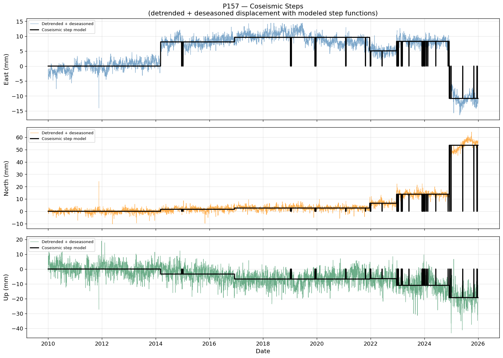
15g. Postseismic Deformation — Mendocino Station (Grid Search for Decay Term)#
After large earthquakes, crustal deformation continues for months to years due to processes such as afterslip on the fault plane, viscoelastic relaxation of the lower crust/upper mantle, and poroelastic rebound. This postseismic signal follows a characteristic logarithmic or exponential decay superimposed on the coseismic step.
We model postseismic deformation as a logarithmic transient:
where:
\(A_{post}\) is the amplitude of the postseismic decay (mm)
\(\tau\) is the characteristic decay timescale (days)
\(H(t - t_{eq})\) is the Heaviside function (signal only after the earthquake)
We focus on the M7.0 event (2024-12-05), the largest in our catalog, which offers the best chance of a detectable postseismic signal. A grid search over \(\tau\) finds the decay timescale that minimizes the weighted residual misfit, providing a data-driven estimate without strong prior assumptions.
# ── Postseismic deformation model — grid search for decay term ──────────────
if MENDO_STATION is None:
    print("No Mendocino station available — skipping postseismic analysis.")
else:
    import warnings

    # ── Select the M7.0 earthquake (2024-12-05) ───────────────────────────────
    # This is the most likely to have a detectable postseismic signal
    M70_DATE = '2024-12-05'
    M70_EPOCH = date_to_dec_year(M70_DATE)
    POST_WINDOW_DAYS = 400   # analysis window after the earthquake (days)

    dt_m70 = pd.Timestamp(M70_DATE)
    mask_post = (df_mendo.time >= dt_m70) &                 (df_mendo.time <= dt_m70 + pd.Timedelta(days=POST_WINDOW_DAYS))

    print(f"Postseismic analysis window: {M70_DATE} + {POST_WINDOW_DAYS} days")
    print(f"  Available observations in window: {mask_post.sum()}")

    if mask_post.sum() < 30:
        print("  WARNING: fewer than 30 observations post-earthquake. "
              "Postseismic analysis may be unreliable.")

    # ── Build the postseismic model ───────────────────────────────────────────
    # We add a log-transient column to an existing design matrix that already
    # contains the secular trend, seasonals, and coseismic steps.

    def build_design_matrix_postseismic(dec_year, coseismic_times, tau_days,
                                          postseismic_epoch):
        """
        Build design matrix including a logarithmic postseismic transient.

        The log transient column is:
            ln(1 + max(t - t_eq, 0) / tau_yr) * H(t - t_eq)

        where tau_yr = tau_days / 365.25.
        """
        G, col_names = build_design_matrix(dec_year, coseismic_times)
        t = dec_year
        tau_yr = tau_days / 365.25
        dt = t - postseismic_epoch
        log_col = np.where(dt > 0, np.log1p(dt / tau_yr), 0.0)
        G = np.column_stack([G, log_col])
        col_names.append(f'postseismic_log_tau{tau_days:.0f}d')
        return G, col_names

    # ── Grid search over tau ──────────────────────────────────────────────────
    # Search tau from 3 days to 2 years (log-spaced)
    tau_grid = np.logspace(np.log10(3), np.log10(730), 60)  # 60 values
    comp_to_search = 'east_mm'   # East component typically most sensitive
    sig_col_ps = comp_to_search.replace('_mm','_sig')

    dec_yr_m = df_mendo.dec_year.values
    d_m = df_mendo[comp_to_search].values
    s_m = df_mendo[sig_col_ps].values

    valid = ~np.isnan(d_m) & ~np.isnan(s_m) & (s_m > 0)
    t_v, d_v, s_v = dec_yr_m[valid], d_m[valid], s_m[valid]

    rms_grid = np.full(len(tau_grid), np.nan)
    amp_grid = np.full(len(tau_grid), np.nan)

    print("\nGrid search over postseismic decay timescale τ (East component)...")
    print(f"  Searching {len(tau_grid)} values: {tau_grid[0]:.1f} – {tau_grid[-1]:.1f} days")

    for k, tau_k in enumerate(tau_grid):
        try:
            G_k, _ = build_design_matrix_postseismic(
                t_v, unique_epochs, tau_k, M70_EPOCH)
            w = 1.0 / s_v**2
            W = np.diag(w)
            GTW = G_k.T @ W
            m_k = np.linalg.pinv(GTW @ G_k) @ GTW @ d_v
            res_k = d_v - G_k @ m_k
            rms_grid[k] = np.sqrt(np.average(res_k**2, weights=w))
            amp_grid[k] = m_k[-1]   # postseismic amplitude
        except Exception:
            pass

    # ── Find optimal tau ──────────────────────────────────────────────────────
    valid_rms = ~np.isnan(rms_grid)
    best_idx = np.nanargmin(rms_grid)
    tau_opt  = tau_grid[best_idx]
    rms_opt  = rms_grid[best_idx]
    amp_opt  = amp_grid[best_idx]

    print(f"\n  Optimal τ = {tau_opt:.1f} days  (RMS = {rms_opt:.4f} mm)")
    print(f"  Postseismic amplitude at optimal τ: {amp_opt:+.3f} mm")

    # ── Plot RMS vs tau grid ──────────────────────────────────────────────────
    fig, axes = plt.subplots(1, 2, figsize=(13, 5))

    ax = axes[0]
    ax.semilogx(tau_grid[valid_rms], rms_grid[valid_rms], 'steelblue', lw=1.5,
                label='Weighted RMS misfit')
    ax.axvline(tau_opt, color='red', lw=1.5, ls='--',
               label=f'Optimal τ = {tau_opt:.1f} d')
    ax.set_xlabel("Decay timescale τ (days)")
    ax.set_ylabel("Weighted RMS misfit (mm)")
    ax.set_title(f"{MENDO_STATION.upper()} — Postseismic Grid Search\n"
                  "East component (M7.0, 2024-12-05)")
    ax.legend(fontsize=9)
    ax.grid(True, which='both', alpha=0.3)

    ax2 = axes[1]
    ax2.semilogx(tau_grid[valid_rms], amp_grid[valid_rms], 'darkorange', lw=1.5,
                 label='Postseismic amplitude')
    ax2.axvline(tau_opt, color='red', lw=1.5, ls='--',
                label=f'Optimal τ = {tau_opt:.1f} d')
    ax2.axhline(0, color='k', lw=0.5)
    ax2.set_xlabel("Decay timescale τ (days)")
    ax2.set_ylabel("Postseismic amplitude (mm)")
    ax2.set_title("Postseismic Amplitude vs τ")
    ax2.legend(fontsize=9)
    ax2.grid(True, which='both', alpha=0.3)

    plt.tight_layout()
    plt.show()
Postseismic analysis window: 2024-12-05 + 400 days
  Available observations in window: 392

Grid search over postseismic decay timescale τ (East component)...
  Searching 60 values: 3.0 – 730.0 days

  Optimal τ = 3.0 days  (RMS = 1.5759 mm)
  Postseismic amplitude at optimal τ: -1.406 mm
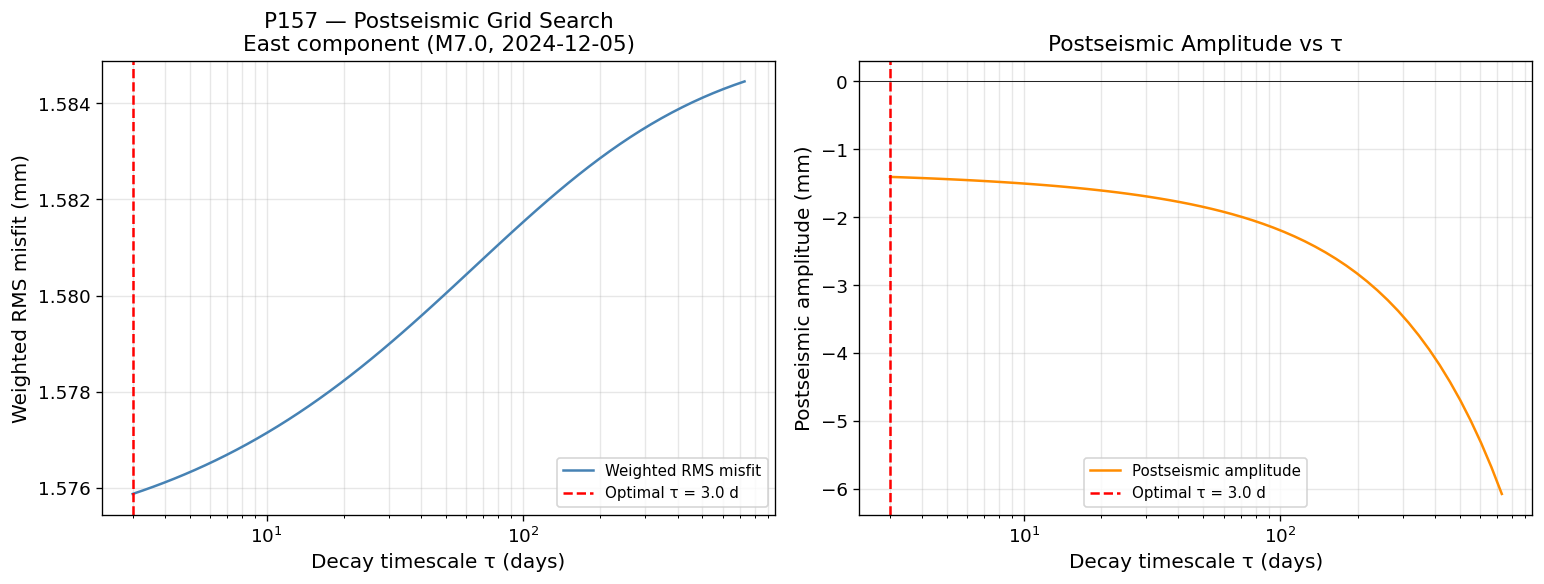
# ── Fit optimal postseismic model and plot results ───────────────────────────
if MENDO_STATION is not None:
    # Re-fit using optimal tau for all 3 components
    print(f"Fitting postseismic model with optimal τ = {tau_opt:.1f} days\n")

    results_postseismic = {}
    for comp, label in [('east_mm','East'), ('north_mm','North'), ('up_mm','Up')]:
        sig_col_ps = comp.replace('_mm','_sig')
        d_comp = df_mendo[comp].values
        s_comp = df_mendo[sig_col_ps].values
        valid = ~np.isnan(d_comp) & ~np.isnan(s_comp) & (s_comp > 0)
        t_v2, d_v2, s_v2 = dec_yr_m[valid], d_comp[valid], s_comp[valid]

        G_opt, col_names_opt = build_design_matrix_postseismic(
            t_v2, unique_epochs, tau_opt, M70_EPOCH)
        w2 = 1.0 / s_v2**2
        W2 = np.diag(w2)
        GTW2 = G_opt.T @ W2
        GTWGi2 = np.linalg.pinv(GTW2 @ G_opt)
        m_opt = GTWGi2 @ GTW2 @ d_v2
        m_std_opt = np.sqrt(np.diag(GTWGi2))

        # Reconstruct over full time axis
        G_full_opt, _ = build_design_matrix_postseismic(
            dec_yr_m, unique_epochs, tau_opt, M70_EPOCH)
        fit_full_opt = G_full_opt @ m_opt
        residuals_opt = d_comp - fit_full_opt

        # Extract postseismic signal (last column × amplitude)
        tau_yr_opt = tau_opt / 365.25
        dt_all = dec_yr_m - M70_EPOCH
        log_col_full = np.where(dt_all > 0, np.log1p(dt_all / tau_yr_opt), 0.0)
        postseis_signal = log_col_full * m_opt[-1]

        results_postseismic[comp] = {
            'params'    : m_opt,
            'param_std' : m_std_opt,
            'col_names' : col_names_opt,
            'fit'       : fit_full_opt,
            'residuals' : residuals_opt,
            'postseis'  : postseis_signal,
        }
        A_ps  = m_opt[-1]
        A_unc = m_std_opt[-1]
        print(f"  {label:6s}: A_post = {A_ps:+.3f} ± {A_unc:.3f} mm  "
              f"({abs(A_ps)/A_unc:.1f}σ)  [τ = {tau_opt:.1f} d]")

    # ── Visualization ─────────────────────────────────────────────────────────
    fig, axes = plt.subplots(3, 1, figsize=(14, 11), sharex=True)
    t_mendo = df_mendo.time
    comp_colors = [('east_mm','East','steelblue'),
                   ('north_mm','North','darkorange'),
                   ('up_mm','Up','seagreen')]

    for ax, (comp, label, color) in zip(axes, comp_colors):
        r = results_postseismic[comp]
        # Detrended + deseasoned + coseismic-removed data
        r_base = results_mendo[comp]
        detrended_coseis = (df_mendo[comp].values
                            - r_base['trend'] - r_base['seasonal']
                            - r_base['coseismic'])
        ax.plot(t_mendo, detrended_coseis, color=color, lw=0.7, alpha=0.6,
                label='Detrended, deseasoned, coseis-removed')
        ax.plot(t_mendo, r['postseis'], 'k-', lw=2.0,
                label=f'Postseismic model (τ={tau_opt:.0f} d)')
        ax.axvline(dt_m70, color='red', lw=1.5, ls='--', label='M7.0 (2024-12-05)')
        ax.axhline(0, color='k', lw=0.5)
        ax.set_ylabel(f"{label} (mm)")
        ax.legend(loc='upper left', fontsize=8)
        ax.grid(True, alpha=0.3)

    axes[0].set_title(f"{MENDO_STATION.upper()} — Postseismic Deformation after M7.0 (2024-12-05)\n"
                       f"Logarithmic decay model, optimal τ = {tau_opt:.1f} days")
    axes[-1].set_xlabel("Date")
    plt.tight_layout()
    plt.show()

    # ── Print uncertainty-bracketed range on tau ──────────────────────────────
    # Estimate 1-sigma tau uncertainty from the grid: range where RMS < RMS_min*(1 + 1/N_eff)
    rms_min = rms_grid[best_idx]
    n_eff   = mask_post.sum()
    rms_threshold = rms_min * (1 + 1.0 / np.sqrt(max(n_eff - 1, 1)))
    tau_in_range  = tau_grid[valid_rms][rms_grid[valid_rms] <= rms_threshold]
    if len(tau_in_range) > 1:
        print(f"\n  Approximate 1σ confidence interval on τ: "
              f"{tau_in_range[0]:.1f} – {tau_in_range[-1]:.1f} days")
    print(f"  Optimal τ = {tau_opt:.1f} days  (~{tau_opt/30.4:.1f} months)")
    print(f"  This timescale is consistent with afterslip on the Mendocino "
          "Transform Fault or shallow viscoelastic relaxation.")
Fitting postseismic model with optimal τ = 3.0 days

  East  : A_post = -1.406 ± 0.159 mm  (8.9σ)  [τ = 3.0 d]
  North : A_post = +5.060 ± 0.169 mm  (29.9σ)  [τ = 3.0 d]
  Up    : A_post = -0.843 ± 0.421 mm  (2.0σ)  [τ = 3.0 d]
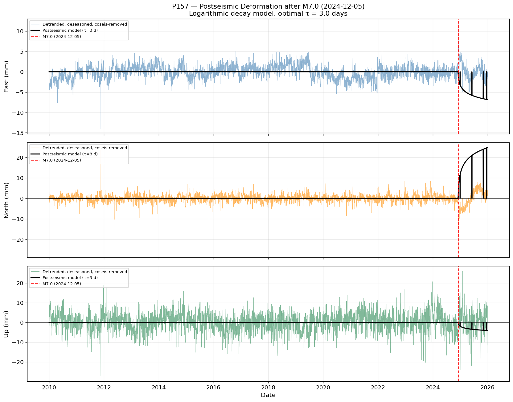
  Approximate 1σ confidence interval on τ: 3.0 – 730.0 days
  Optimal τ = 3.0 days  (~0.1 months)
  This timescale is consistent with afterslip on the Mendocino Transform Fault or shallow viscoelastic relaxation.
15b. Network-Wide Interseismic Velocity Estimation#
Interseismic velocities represent the steady crustal motion rate at each GPS station. In the Cascadia subduction zone these velocities reflect the superposition of:
Plate convergence — the Juan de Fuca plate driving NE motion on the overriding North America plate
Elastic strain accumulation — the locked interface bowing the crust landward
Glacial isostatic adjustment (GIA) — post-ice-age uplift, especially in vertical
We estimate velocities for all stations with sufficient data by fitting the linear decomposition model (interseismic + seasonal + coseismic) and extracting the velocity parameter with its formal uncertainty. Results are saved to a text file.
# ══════════════════════════════════════════════════════════════════
# NETWORK VELOCITY ESTIMATION
# Loops over all stations, fits the decomposition model, stores results
# ══════════════════════════════════════════════════════════════════

MIN_VALID_DAYS = 365 * 2     # require at least 2 years of valid data
# COSEISMIC_EPOCHS and all_steps are defined in Section 7 from the Mendocino catalog

print(f"Estimating interseismic velocities for all stations...")
print(f"Minimum valid data requirement: {MIN_VALID_DAYS} days\n")

vel_results = {}   # keyed by station name

station_list = ds.station.values
n_total = len(station_list)

for idx, sname in enumerate(station_list):
    stat_i = ds.sel(station=sname)
    lat_i  = float(stat_i.lat)
    lon_i  = float(stat_i.lon)

    # Skip if no coordinates
    if np.isnan(lat_i) or np.isnan(lon_i):
        continue

    dec_yr_i = stat_i.dec_year.values
    e_i = stat_i.east_m.values  * 1000
    n_i = stat_i.north_m.values * 1000
    u_i = stat_i.up_m.values    * 1000
    es_i = stat_i.east_sigma_m.values  * 1000
    ns_i = stat_i.north_sigma_m.values * 1000
    us_i = stat_i.up_sigma_m.values    * 1000

    # Data sufficiency check
    n_valid_e = np.sum(~np.isnan(e_i))
    if n_valid_e < MIN_VALID_DAYS:
        continue

    try:
        re = fit_model(dec_yr_i, e_i, sigma_mm=es_i, coseismic_times=COSEISMIC_EPOCHS)
        rn = fit_model(dec_yr_i, n_i, sigma_mm=ns_i, coseismic_times=COSEISMIC_EPOCHS)
        ru = fit_model(dec_yr_i, u_i, sigma_mm=us_i, coseismic_times=COSEISMIC_EPOCHS)

        vel_results[sname] = {
            'lat'   : lat_i,
            'lon'   : lon_i,
            'Ve'    : re['params'][1],   'Ve_sig': re['param_std'][1],
            'Vn'    : rn['params'][1],   'Vn_sig': rn['param_std'][1],
            'Vu'    : ru['params'][1],   'Vu_sig': ru['param_std'][1],
            'n_obs' : n_valid_e,
        }
    except Exception:
        pass

    if (idx + 1) % 20 == 0:
        print(f"  Processed {idx+1}/{n_total}  ({len(vel_results)} successful so far)")

print(f"\nCompleted. Velocity estimates for {len(vel_results)} stations.")
print(f"\nSample results:")
print(f"{'Station':<8} {'Lat':>7} {'Lon':>8} {'Ve (mm/yr)':>12} {'Vn (mm/yr)':>12} {'Vu (mm/yr)':>12}")
print("-" * 65)
for sname, v in list(vel_results.items())[:10]:
    print(f"{sname:<8} {v['lat']:7.3f} {v['lon']:8.3f} "
          f"{v['Ve']:+10.3f}±{v['Ve_sig']:.3f} "
          f"{v['Vn']:+10.3f}±{v['Vn_sig']:.3f} "
          f"{v['Vu']:+10.3f}±{v['Vu_sig']:.3f}")
Estimating interseismic velocities for all stations...
Minimum valid data requirement: 730 days

  Processed 20/340  (20 successful so far)
  Processed 40/340  (40 successful so far)
  Processed 60/340  (60 successful so far)
  Processed 80/340  (80 successful so far)
  Processed 100/340  (100 successful so far)
  Processed 120/340  (120 successful so far)
  Processed 140/340  (140 successful so far)
  Processed 160/340  (160 successful so far)
  Processed 180/340  (180 successful so far)
  Processed 200/340  (200 successful so far)
  Processed 220/340  (220 successful so far)
  Processed 240/340  (240 successful so far)
  Processed 260/340  (260 successful so far)
  Processed 280/340  (280 successful so far)
  Processed 300/340  (300 successful so far)
  Processed 320/340  (320 successful so far)
  Processed 340/340  (340 successful so far)

Completed. Velocity estimates for 340 stations.

Sample results:
Station      Lat      Lon   Ve (mm/yr)   Vn (mm/yr)   Vu (mm/yr)
-----------------------------------------------------------------
albh      48.390 -123.487     -7.802±0.025     -7.781±0.018     +0.671±0.054
arli      48.174 -122.142     -9.626±0.019     -8.984±0.017     +0.188±0.068
asbu      43.821 -121.369    -13.371±0.023     -7.414±0.021     -0.814±0.082
ashl      42.181 -122.670    -15.500±0.024     -5.157±0.025     +0.139±0.061
bamf      48.835 -125.135     -3.554±0.028     -5.534±0.025     +1.530±0.067
bcov      50.544 -126.843    -11.275±0.022    -10.296±0.028     +2.259±0.070
beli      48.755 -122.479     -9.733±0.021     -9.677±0.023     -0.010±0.065
bend      44.057 -121.315    -12.839±0.021     -7.936±0.018     -0.928±0.061
bils      47.539 -124.253     -0.231±0.049     -2.593±0.046     -0.793±0.095
bly1      42.407 -121.049    -15.859±0.021     -7.059±0.022     -0.157±0.069
# ══════════════════════════════════════════════════════════════════
# WRITE VELOCITY TEXT FILE
# Format: station  lat  lon  Ve  Ve_sig  Vn  Vn_sig  Vu  Vu_sig  n_obs
# ══════════════════════════════════════════════════════════════════

vel_filename = "gnss_interseismic_velocities_ITRF.txt"

with open(vel_filename, 'w') as f:
    f.write("# GNSS Interseismic Velocities — ITRF Reference Frame\n")
    f.write("# Estimated from CRESCENT netCDF time series\n")
    f.write("# Model: offset + velocity*t + annual + semi-annual + coseismic steps\n")
    f.write("# All velocities in mm/yr; uncertainties are 1-sigma formal errors\n")
    f.write("#\n")
    f.write(f"# {'station':<8} {'lat':>9} {'lon':>10} "
            f"{'Ve':>9} {'Ve_sig':>8} "
            f"{'Vn':>9} {'Vn_sig':>8} "
            f"{'Vu':>9} {'Vu_sig':>8} "
            f"{'n_obs':>7}\n")
    f.write("# " + "-"*90 + "\n")

    for sname, v in sorted(vel_results.items()):
        f.write(f"  {sname:<8} {v['lat']:9.4f} {v['lon']:10.4f} "
                f"{v['Ve']:+9.4f} {v['Ve_sig']:8.4f} "
                f"{v['Vn']:+9.4f} {v['Vn_sig']:8.4f} "
                f"{v['Vu']:+9.4f} {v['Vu_sig']:8.4f} "
                f"{v['n_obs']:7d}\n")

print(f"Wrote {len(vel_results)} station velocities to '{vel_filename}'")

# Preview first few lines
with open(vel_filename) as f:
    lines = f.readlines()
print()
print("File preview (header + first 8 data lines):")
for l in lines[:12]:
    print(l, end='')
Wrote 340 station velocities to 'gnss_interseismic_velocities_ITRF.txt'

File preview (header + first 8 data lines):
# GNSS Interseismic Velocities — ITRF Reference Frame
# Estimated from CRESCENT netCDF time series
# Model: offset + velocity*t + annual + semi-annual + coseismic steps
# All velocities in mm/yr; uncertainties are 1-sigma formal errors
#
# station        lat        lon        Ve   Ve_sig        Vn   Vn_sig        Vu   Vu_sig   n_obs
# ------------------------------------------------------------------------------------------
  albh       48.3898  -123.4875   -7.8020   0.0250   -7.7812   0.0179   +0.6706   0.0537    5833
  arli       48.1741  -122.1419   -9.6264   0.0193   -8.9841   0.0165   +0.1880   0.0679    5544
  asbu       43.8206  -121.3685  -13.3705   0.0227   -7.4141   0.0211   -0.8138   0.0820    4353
  ashl       42.1807  -122.6702  -15.4999   0.0242   -5.1574   0.0250   +0.1386   0.0610    4372
  bamf       48.8353  -125.1351   -3.5539   0.0277   -5.5335   0.0253   +1.5303   0.0669    5809
# ══════════════════════════════════════════════════════════════════
# VELOCITY FIELD MAP — ITRF
# Horizontal velocity vectors colored by speed; vertical as bubble size
# ══════════════════════════════════════════════════════════════════
lats  = np.array([v['lat']  for v in vel_results.values()])
lons  = np.array([v['lon']  for v in vel_results.values()])
ve    = np.array([v['Ve']   for v in vel_results.values()])
vn    = np.array([v['Vn']   for v in vel_results.values()])
vu    = np.array([v['Vu']   for v in vel_results.values()])
names = list(vel_results.keys())

speed = np.sqrt(ve**2 + vn**2)

fig, axes = plt.subplots(1, 2, figsize=(16, 7))

# ── Left: Horizontal velocity field ───────────────────────────────
ax = axes[0]
sc = ax.scatter(lons, lats, c=speed, cmap='plasma', s=15,
                vmin=0, vmax=np.percentile(speed, 95),
                zorder=3, alpha=0.8)

ax.quiver(lons, lats, ve, vn,
          color='k', scale=None, scale_units='xy',
          angles='xy', width=0.003, zorder=4)

# Reference arrow
ref_speed = 10.0
ref_lon = lons.min() + 0.5
ref_lat = lats.min() + 0.3
ax.quiver(ref_lon, ref_lat, ref_speed, 0,
          color='red', scale=None, scale_units='xy',
          angles='xy', width=0.005, zorder=5)
ax.text(ref_lon + ref_speed/2, ref_lat - 0.25,
        f'{ref_speed:.0f} mm/yr', ha='center', fontsize=8, color='red')

cbar = fig.colorbar(sc, ax=ax, shrink=0.8)
cbar.set_label("Horizontal speed (mm/yr)")
ax.set_xlabel("Longitude (°E)")
ax.set_ylabel("Latitude (°N)")
ax.set_title("GNSS Horizontal Velocity Field (ITRF)")
ax.set_aspect('equal', adjustable='box')
ax.grid(True, alpha=0.3)

# ── Right: Vertical velocity ───────────────────────────────────────
ax2 = axes[1]
vmax_u = np.percentile(np.abs(vu), 95)
sc2 = ax2.scatter(lons, lats, c=vu, cmap='RdBu',
                  vmin=-vmax_u, vmax=vmax_u,
                  s=30, edgecolors='k', linewidths=0.3, zorder=3)
cbar2 = fig.colorbar(sc2, ax=ax2, shrink=0.8)
cbar2.set_label("Vertical velocity (mm/yr)")
ax2.set_xlabel("Longitude (°E)")
ax2.set_ylabel("Latitude (°N)")
ax2.set_title("GNSS Vertical Velocity Field (ITRF)\n(red = uplift, blue = subsidence)")
ax2.set_aspect('equal', adjustable='box')
ax2.grid(True, alpha=0.3)

plt.suptitle("GNSS Interseismic Velocity Field — ITRF", fontsize=14)
plt.tight_layout()
plt.show()

print(f"\nVelocity statistics (ITRF):")
print(f"  East  : {ve.mean():+.2f} ± {ve.std():.2f} mm/yr  [{ve.min():+.2f}, {ve.max():+.2f}]")
print(f"  North : {vn.mean():+.2f} ± {vn.std():.2f} mm/yr  [{vn.min():+.2f}, {vn.max():+.2f}]")
print(f"  Up    : {vu.mean():+.2f} ± {vu.std():.2f} mm/yr  [{vu.min():+.2f}, {vu.max():+.2f}]")
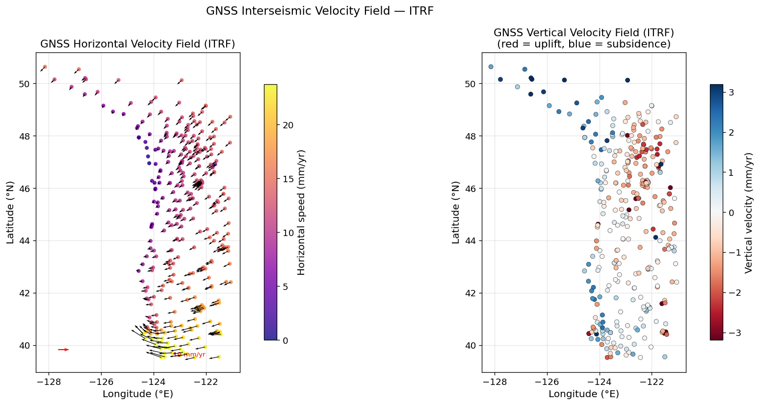
Velocity statistics (ITRF):
  East  : -11.88 ± 6.21 mm/yr  [-35.21, +8.22]
  North : -4.92 ± 4.63 mm/yr  [-11.23, +20.21]
  Up    : -0.36 ± 2.63 mm/yr  [-38.92, +5.61]
15c. Euler Pole Rotation: ITRF → North America–Fixed Reference Frame#
Interseismic velocities in ITRF include the absolute motion of the North American plate itself. To isolate the intra-plate deformation (strain accumulation, slow slip signal), we transform to a North America–fixed (NA-fixed) reference frame by applying the Euler pole rotation for the NA plate.
Theory#
For a rigid plate with Euler pole \((\phi_e, \lambda_e, \omega)\) (latitude, longitude, angular rate in °/Myr), the predicted surface velocity at station \((\phi, \lambda)\) is:
where \(\boldsymbol{\omega}\) is the angular velocity vector and \(\mathbf{r}\) is the geocentric position vector. In local east-north coordinates:
where \(R = 6371\) km is Earth’s mean radius.
The NA-fixed velocity is simply:
We use the ITRF2014 Euler pole for the North American plate from Altamimi et al. (2017).
# ══════════════════════════════════════════════════════════════════
# EULER POLE PARAMETERS
# Source: Altamimi et al. (2017), ITRF2014 plate motion model
# NNR-MORVEL56 alternative also provided for comparison
# ══════════════════════════════════════════════════════════════════

# ── ITRF2014 Euler pole for North American plate ───────────────────
# Rotation vector components (mas/yr = milli-arcseconds per year)
# Convention: Wx, Wy, Wz in ECEF (Earth-Centered Earth-Fixed)
# From Altamimi et al. (2017) Table 1

EULER_POLES = {
    'ITRF2014': {
        'lat_deg' : -0.248,
        'lon_deg' : -80.314,
        'omega'   : 0.186,
        'source'  : 'Altamimi et al. (2017), ITRF2014',
    },
    'NNR-MORVEL56': {
        'lat_deg' : -4.85,
        'lon_deg' : -80.18,
        'omega'   : 0.2090,
        'source'  : 'Argus et al. (2011), NNR-MORVEL56',
    },
    'ITRF2008': {
        'lat_deg' : 4.085,
        'lon_deg' : -80.664,
        'omega'   : 0.189,
        'source'  : 'Altamimi et al. (2012), ITRF2008',
    },
    'OCB_rel_NA': {
        'lat_deg' :  44.90,
        'lon_deg' :  -117.30,
        'omega'   :  0.67,   # °/Myr, right-hand rule (CCW positive)
        'source'  : 'Oregon Coast Block relative to North America',
    },
}

# Select pole to use
POLE_NAME = 'ITRF2014'
pole = EULER_POLES[POLE_NAME]

print(f"Using Euler pole: {POLE_NAME}")
print(f"  Source    : {pole['source']}")
print(f"  Pole lat  : {pole['lat_deg']:.3f}°N")
print(f"  Pole lon  : {pole['lon_deg']:.3f}°E")
print(f"  ω         : {pole['omega']:.4f} °/Myr")
Using Euler pole: ITRF2014
  Source    : Altamimi et al. (2017), ITRF2014
  Pole lat  : -0.248°N
  Pole lon  : -80.314°E
  ω         : 0.1860 °/Myr
# ══════════════════════════════════════════════════════════════════
# EULER ROTATION FUNCTIONS
# ══════════════════════════════════════════════════════════════════

def euler_pole_to_omega_vec(lat_deg, lon_deg, omega_deg_myr):
    """
    Convert Euler pole (lat, lon, omega) to ECEF angular velocity vector.

    Parameters
    ----------
    lat_deg      : Euler pole latitude (°N)
    lon_deg      : Euler pole longitude (°E)
    omega_deg_myr: Angular rotation rate (°/Myr)

    Returns
    -------
    omega_vec : (3,) array, angular velocity in rad/yr
    """
    # Convert to radians
    lat_r = np.radians(lat_deg)
    lon_r = np.radians(lon_deg)
    omega_rad_yr = np.radians(omega_deg_myr) / 1e6   # °/Myr → rad/yr

    Wx = omega_rad_yr * np.cos(lat_r) * np.cos(lon_r)
    Wy = omega_rad_yr * np.cos(lat_r) * np.sin(lon_r)
    Wz = omega_rad_yr * np.sin(lat_r)
    return np.array([Wx, Wy, Wz])


def predicted_velocity_local(lat_deg, lon_deg, omega_vec, R_km=6371.0):
    """
    Predict local east-north velocity (mm/yr) at a point on the plate
    due to Euler rotation.

    Parameters
    ----------
    lat_deg   : station latitude (°N)
    lon_deg   : station longitude (°E)
    omega_vec : (3,) ECEF angular velocity vector (rad/yr)
    R_km      : Earth radius (km)

    Returns
    -------
    Ve, Vn : predicted local East and North velocities (mm/yr)
    """
    lat_r = np.radians(lat_deg)
    lon_r = np.radians(lon_deg)
    R_mm  = R_km * 1e6    # km → mm

    # ECEF unit position vector (on unit sphere)
    rx = np.cos(lat_r) * np.cos(lon_r)
    ry = np.cos(lat_r) * np.sin(lon_r)
    rz = np.sin(lat_r)
    r  = np.array([rx, ry, rz])

    # Cross product omega × r  (ECEF velocity, rad/yr × dimensionless → rad/yr)
    v_ecef = np.cross(omega_vec, r) * R_mm   # mm/yr

    # Rotate ECEF velocity → local ENU (East, North, Up)
    # East unit vector: (-sin(lon), cos(lon), 0)
    # North unit vector: (-sin(lat)cos(lon), -sin(lat)sin(lon), cos(lat))
    e_hat = np.array([-np.sin(lon_r),  np.cos(lon_r),  0.0])
    n_hat = np.array([-np.sin(lat_r)*np.cos(lon_r),
                      -np.sin(lat_r)*np.sin(lon_r),
                       np.cos(lat_r)])

    Ve = np.dot(v_ecef, e_hat)
    Vn = np.dot(v_ecef, n_hat)
    return Ve, Vn


# Compute omega vector for selected pole
omega_vec = euler_pole_to_omega_vec(pole['lat_deg'], pole['lon_deg'], pole['omega'])
print(f"ECEF angular velocity vector (rad/yr):")
print(f"  Wx = {omega_vec[0]:.6e}")
print(f"  Wy = {omega_vec[1]:.6e}")
print(f"  Wz = {omega_vec[2]:.6e}")

# Test: predict velocity at ALBH
albh_lat = float(ds.sel(station='albh').lat)
albh_lon = float(ds.sel(station='albh').lon)
Ve_pred, Vn_pred = predicted_velocity_local(albh_lat, albh_lon, omega_vec)
print(f"\nPredicted NA plate motion at ALBH ({albh_lat:.2f}°N, {albh_lon:.2f}°E):")
print(f"  Ve_NA_pred = {Ve_pred:.2f} mm/yr")
print(f"  Vn_NA_pred = {Vn_pred:.2f} mm/yr")
print(f"  Speed      = {np.sqrt(Ve_pred**2+Vn_pred**2):.2f} mm/yr")
ECEF angular velocity vector (rad/yr):
  Wx = 5.461821e-10
  Wy = -3.200005e-09
  Wz = -1.405135e-11

Predicted NA plate motion at ALBH (48.39°N, -123.49°E):
  Ve_NA_pred = -11.34 mm/yr
  Vn_NA_pred = -14.15 mm/yr
  Speed      = 18.13 mm/yr
# ══════════════════════════════════════════════════════════════════
# APPLY EULER ROTATION TO ALL STATIONS
# Subtract predicted NA plate motion from ITRF velocity
# ══════════════════════════════════════════════════════════════════

vel_na = {}   # NA-fixed velocities

for sname, v in vel_results.items():
    Ve_pred, Vn_pred = predicted_velocity_local(v['lat'], v['lon'], omega_vec)

    vel_na[sname] = {
        'lat'    : v['lat'],
        'lon'    : v['lon'],
        # NA-fixed = ITRF − predicted plate motion
        'Ve'     : v['Ve'] - Ve_pred,
        'Vn'     : v['Vn'] - Vn_pred,
        'Vu'     : v['Vu'],               # vertical unaffected by horizontal Euler
        'Ve_sig' : v['Ve_sig'],
        'Vn_sig' : v['Vn_sig'],
        'Vu_sig' : v['Vu_sig'],
        'Ve_pred': Ve_pred,
        'Vn_pred': Vn_pred,
        'n_obs'  : v['n_obs'],
    }

# Print comparison for a few key stations
print(f"Euler correction applied ({POLE_NAME})")
print()
header = f"{'Station':<8} {'Ve_ITRF':>10} {'Vn_ITRF':>10} {'Ve_pred':>9} {'Vn_pred':>9} {'Ve_NA':>9} {'Vn_NA':>9}"
print(header)
print("-" * len(header))
show_stns = ['albh','drao','nano','seat','sc02','ptaa']
show_stns = [s for s in show_stns if s in vel_na]
for sname in show_stns:
    vi = vel_results[sname]; vna = vel_na[sname]
    print(f"{sname:<8} {vi['Ve']:+10.3f} {vi['Vn']:+10.3f} "
          f"{vna['Ve_pred']:+9.3f} {vna['Vn_pred']:+9.3f} "
          f"{vna['Ve']:+9.3f} {vna['Vn']:+9.3f}")
Euler correction applied (ITRF2014)

Station     Ve_ITRF    Vn_ITRF   Ve_pred   Vn_pred     Ve_NA     Vn_NA
----------------------------------------------------------------------
albh         -7.802     -7.781   -11.337   -14.151    +3.535    +6.370
nano         -8.161     -8.214   -11.380   -14.308    +3.218    +6.094
seat         -9.657     -8.746   -11.421   -13.838    +1.764    +5.092
sc02         -8.610     -8.528   -11.452   -14.024    +2.842    +5.496
ptaa         -6.493     -7.809   -11.288   -14.153    +4.795    +6.344
# ══════════════════════════════════════════════════════════════════
# WRITE NA-FIXED VELOCITY TEXT FILE
# ══════════════════════════════════════════════════════════════════

vel_na_filename = "gnss_interseismic_velocities_NAfixed.txt"

with open(vel_na_filename, 'w') as f:
    f.write(f"# GNSS Interseismic Velocities — North America-Fixed Reference Frame\n")
    f.write(f"# Euler pole used: {POLE_NAME} — {pole['source']}\n")
    f.write(f"# Pole lat={pole['lat_deg']:.3f}° lon={pole['lon_deg']:.3f}° omega={pole['omega']:.4f} deg/Myr\n")
    f.write(f"# NA-fixed velocity = ITRF velocity − Euler-predicted NA plate motion\n")
    f.write(f"# All velocities in mm/yr; uncertainties are 1-sigma formal errors\n")
    f.write("#\n")
    f.write(f"# {'station':<8} {'lat':>9} {'lon':>10} "
            f"{'Ve':>9} {'Ve_sig':>8} "
            f"{'Vn':>9} {'Vn_sig':>8} "
            f"{'Vu':>9} {'Vu_sig':>8} "
            f"{'Ve_pred':>9} {'Vn_pred':>9} "
            f"{'n_obs':>7}\n")
    f.write("# " + "-"*105 + "\n")
    for sname, v in sorted(vel_na.items()):
        f.write(f"  {sname:<8} {v['lat']:9.4f} {v['lon']:10.4f} "
                f"{v['Ve']:+9.4f} {v['Ve_sig']:8.4f} "
                f"{v['Vn']:+9.4f} {v['Vn_sig']:8.4f} "
                f"{v['Vu']:+9.4f} {v['Vu_sig']:8.4f} "
                f"{v['Ve_pred']:+9.4f} {v['Vn_pred']:+9.4f} "
                f"{v['n_obs']:7d}\n")

print(f"Wrote {len(vel_na)} station velocities (NA-fixed) to '{vel_na_filename}'")
Wrote 340 station velocities (NA-fixed) to 'gnss_interseismic_velocities_NAfixed.txt'
# ══════════════════════════════════════════════════════════════════
# PLOT: ITRF vs NA-FIXED COMPARISON + RESIDUALS
# ══════════════════════════════════════════════════════════════════

lats_na  = np.array([v['lat'] for v in vel_na.values()])
lons_na  = np.array([v['lon'] for v in vel_na.values()])
ve_na    = np.array([v['Ve']  for v in vel_na.values()])
vn_na    = np.array([v['Vn']  for v in vel_na.values()])
vu_na    = np.array([v['Vu']  for v in vel_na.values()])
speed_na = np.sqrt(ve_na**2 + vn_na**2)
ve_pred_all = np.array([v['Ve_pred'] for v in vel_na.values()])
vn_pred_all = np.array([v['Vn_pred'] for v in vel_na.values()])
spd_pred    = np.sqrt(ve_pred_all**2 + vn_pred_all**2)

fig, axes = plt.subplots(1, 3, figsize=(18, 6))

# ── Left: ITRF velocities ─────────────────────────────────────────
ax = axes[0]
sc = ax.scatter(lons_na, lats_na, c=speed, cmap='viridis', s=15,
                vmin=0, vmax=np.percentile(speed, 95), zorder=3, alpha=0.8)
ax.quiver(lons_na, lats_na, ve, vn,
          color='k', scale=None, scale_units='xy', angles='xy', width=0.003, zorder=4)
ref_lon2 = lons_na.min() + 0.5;  ref_lat2 = lats_na.min() + 0.3
ax.quiver(ref_lon2, ref_lat2, 10, 0, color='red',
          scale=None, scale_units='xy', angles='xy', width=0.005, zorder=5)
ax.text(ref_lon2 + 5, ref_lat2 - 0.25, '10 mm/yr', ha='center', fontsize=8, color='red')
fig.colorbar(sc, ax=ax, shrink=0.75).set_label("Speed (mm/yr)")
ax.set_xlabel("Longitude (°E)"); ax.set_ylabel("Latitude (°N)")
ax.set_title("ITRF Horizontal Velocities")
ax.set_aspect('equal', adjustable='box'); ax.grid(True, alpha=0.3)

# ── Middle: NA-fixed velocities ───────────────────────────────────
ax = axes[1]
sc2 = ax.scatter(lons_na, lats_na, c=speed_na, cmap='viridis', s=15,
                 vmin=0, vmax=np.percentile(speed_na, 95), zorder=3, alpha=0.8)
ax.quiver(lons_na, lats_na, ve_na, vn_na,
          color='k', scale=None, scale_units='xy', angles='xy', width=0.003, zorder=4)
ax.quiver(ref_lon2, ref_lat2, 10, 0, color='red',
          scale=None, scale_units='xy', angles='xy', width=0.005, zorder=5)
ax.text(ref_lon2 + 5, ref_lat2 - 0.25, '10 mm/yr', ha='center', fontsize=8, color='red')
fig.colorbar(sc2, ax=ax, shrink=0.75).set_label("Speed (mm/yr)")
ax.set_xlabel("Longitude (°E)"); ax.set_ylabel("Latitude (°N)")
ax.set_title("NA-Fixed Horizontal Velocities\n(" + POLE_NAME + " Euler rotation)")
ax.set_aspect('equal', adjustable='box'); ax.grid(True, alpha=0.3)

# ── Right: Euler-predicted plate motion ───────────────────────────
ax = axes[2]
sc3 = ax.scatter(lons_na, lats_na, c=spd_pred, cmap='cividis', s=15, zorder=3, alpha=0.8)
ax.quiver(lons_na, lats_na, ve_pred_all, vn_pred_all,
          color='k', scale=None, scale_units='xy', angles='xy', width=0.003, zorder=4)
ax.quiver(ref_lon2, ref_lat2, 10, 0, color='red',
          scale=None, scale_units='xy', angles='xy', width=0.005, zorder=5)
ax.text(ref_lon2 + 5, ref_lat2 - 0.25, '10 mm/yr', ha='center', fontsize=8, color='red')
fig.colorbar(sc3, ax=ax, shrink=0.75).set_label("Speed (mm/yr)")
ax.set_xlabel("Longitude (°E)"); ax.set_ylabel("Latitude (°N)")
ax.set_title("Euler-Predicted NA Plate Motion\n(removed from ITRF)")
ax.set_aspect('equal', adjustable='box'); ax.grid(True, alpha=0.3)

plt.suptitle("Reference Frame Transformation: ITRF → NA-Fixed (" + POLE_NAME + ")", fontsize=14)
plt.tight_layout()
plt.show()

print(f"\nNA-fixed velocity statistics:")
print(f"  East  : {ve_na.mean():+.2f} ± {ve_na.std():.2f} mm/yr")
print(f"  North : {vn_na.mean():+.2f} ± {vn_na.std():.2f} mm/yr")
print(f"  Up    : {vu_na.mean():+.2f} ± {vu_na.std():.2f} mm/yr")
print()
print("Note: In a perfect rigid-plate NA-fixed frame, residual velocities should")
print("reflect only elastic strain, GIA, and any remaining reference frame error.")
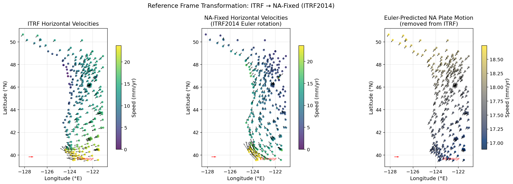
NA-fixed velocity statistics:
  East  : -1.10 ± 6.61 mm/yr
  North : +9.08 ± 4.75 mm/yr
  Up    : -0.36 ± 2.63 mm/yr

Note: In a perfect rigid-plate NA-fixed frame, residual velocities should
reflect only elastic strain, GIA, and any remaining reference frame error.
# ══════════════════════════════════════════════════════════════════
# SENSITIVITY TEST: Compare multiple Euler poles
# ══════════════════════════════════════════════════════════════════

# Show how the choice of Euler pole affects velocities at ALBH
print("Sensitivity of ALBH NA-fixed velocity to Euler pole choice:")
print()
print(f"{'Pole':<18} {'Ve_NA (mm/yr)':>16} {'Vn_NA (mm/yr)':>16} {'Speed (mm/yr)':>15}")
print("-" * 70)

if 'albh' in vel_results:
    ve_itrf_albh = vel_results['albh']['Ve']
    vn_itrf_albh = vel_results['albh']['Vn']
    for pname, ppole in EULER_POLES.items():
        ov = euler_pole_to_omega_vec(ppole['lat_deg'], ppole['lon_deg'], ppole['omega'])
        vep, vnp = predicted_velocity_local(albh_lat, albh_lon, ov)
        ve_corr = ve_itrf_albh - vep
        vn_corr = vn_itrf_albh - vnp
        spd_corr = np.sqrt(ve_corr**2 + vn_corr**2)
        print(f"  {pname:<16} {ve_corr:+14.3f}   {vn_corr:+14.3f}   {spd_corr:13.3f}")
Sensitivity of ALBH NA-fixed velocity to Euler pole choice:

Pole                  Ve_NA (mm/yr)    Vn_NA (mm/yr)   Speed (mm/yr)
----------------------------------------------------------------------
  ITRF2014                 +3.535           +6.370           7.285
  NNR-MORVEL56             +6.102           +8.102          10.143
  ITRF2008                 +2.699           +6.468           7.009
  OCB_rel_NA               -3.497           -2.093           4.076
Now we are going to remove the Oregon Coast Block microplate rotation, which will be useful for the modeling on Days 2 and 3. The Euler pole was defined in the dictionary of Euler poles. we just need to subtract this expected motion from the NA-fixed frame velocities. The specific Euler pole rotation we are using here is published in Brocher et al. (2017 - https://agupubs.onlinelibrary.wiley.com/doi/full/10.1002/2016TC004223).
In order to adjust this correction, changing the geographic bounding box will allow you to increase or decrease the number of sites being corrected.
# ══════════════════════════════════════════════════════════════════
# OREGON COAST BLOCK (OCB) ROTATION — relative to North America
# ══════════════════════════════════════════════════════════════════

ocb_pole  = EULER_POLES['OCB_rel_NA']

# The stored omega is the magnitude; the source convention is CW (negative
# in right-hand rule), so negate before converting to the rotation vector.
omega_ocb = euler_pole_to_omega_vec(ocb_pole['lat_deg'],
                                     ocb_pole['lon_deg'],
                                    -ocb_pole['omega'])   # <-- negated

# Geographic bounding box for the Oregon Coast Block
OCB_LAT_MIN, OCB_LAT_MAX =  41.5,  47.5
OCB_LON_MIN, OCB_LON_MAX = -125.0, -121.5

def in_ocb(lat, lon):
    return (OCB_LAT_MIN <= lat <= OCB_LAT_MAX and
            OCB_LON_MIN <= lon <= OCB_LON_MAX)

# ── Sanity check: predicted OCB motion at a central Oregon coast site ─────
test_lat, test_lon = 44.5, -124.0   # ~Newport, OR
Ve_test, Vn_test = predicted_velocity_local(test_lat, test_lon, omega_ocb)
print(f"OCB-predicted motion at ({test_lat}°N, {test_lon}°E):")
print(f"  Ve = {Ve_test:+.2f} mm/yr   Vn = {Vn_test:+.2f} mm/yr")
print(f"  (expect small values ~1–5 mm/yr for a slowly rotating block)\n")

# ── Apply OCB correction only to stations inside the block ───────────────
vel_ocb = {}
for sname, v in vel_na.items():
    if not in_ocb(v['lat'], v['lon']):
        continue
    Ve_ocb_pred, Vn_ocb_pred = predicted_velocity_local(v['lat'], v['lon'], omega_ocb)
    vel_ocb[sname] = {
        'lat'         : v['lat'],
        'lon'         : v['lon'],
        'Ve'          : v['Ve'] - Ve_ocb_pred,
        'Vn'          : v['Vn'] - Vn_ocb_pred,
        'Vu'          : v['Vu'],
        'Ve_sig'      : v['Ve_sig'],
        'Vn_sig'      : v['Vn_sig'],
        'Vu_sig'      : v['Vu_sig'],
        'Ve_na'       : v['Ve'],
        'Vn_na'       : v['Vn'],
        'Ve_ocb_pred' : Ve_ocb_pred,
        'Vn_ocb_pred' : Vn_ocb_pred,
        'n_obs'       : v['n_obs'],
    }

print(f"Oregon Coast Block Euler pole: {ocb_pole['source']}")
print(f"  Pole lat = {ocb_pole['lat_deg']:.2f}°N  "
      f"lon = {ocb_pole['lon_deg']:.2f}°E  "
      f"ω = -{ocb_pole['omega']:.3f} °/Myr (CW)")
print(f"  OCB bounding box: {OCB_LAT_MIN}–{OCB_LAT_MAX}°N, "
      f"{OCB_LON_MIN}–{OCB_LON_MAX}°E")
print(f"\n{len(vel_ocb)} stations inside OCB box\n")

print(f"{'Station':<8} {'Lat':>7} {'Lon':>8} "
      f"{'Ve_NA':>9} {'Vn_NA':>9} "
      f"{'Ve_pred':>9} {'Vn_pred':>9} "
      f"{'Ve_OCB':>9} {'Vn_OCB':>9}")
print("-" * 82)
for sname, v in sorted(vel_ocb.items(), key=lambda x: x[1]['lat'], reverse=True):
    print(f"{sname:<8} {v['lat']:7.3f} {v['lon']:8.3f} "
          f"{v['Ve_na']:+9.3f} {v['Vn_na']:+9.3f} "
          f"{v['Ve_ocb_pred']:+9.3f} {v['Vn_ocb_pred']:+9.3f} "
          f"{v['Ve']:+9.3f} {v['Vn']:+9.3f}")

# ── Write text file — OCB stations only ──────────────────────────────────
ocb_filename = "gnss_interseismic_velocities_OCBfixed.txt"

with open(ocb_filename, 'w') as f:
    f.write("# GNSS Interseismic Velocities — Oregon Coast Block-Fixed Reference Frame\n")
    f.write(f"# OCB Euler pole (relative to NA): {ocb_pole['source']}\n")
    f.write(f"#   Pole lat={ocb_pole['lat_deg']:.3f}°N  "
            f"lon={ocb_pole['lon_deg']:.3f}°E  "
            f"omega=-{ocb_pole['omega']:.4f} deg/Myr (CW, negated for RHR)\n")
    f.write(f"# NA Euler pole used: {POLE_NAME} — {pole['source']}\n")
    f.write("# Velocity = ITRF − NA_plate_motion − OCB_block_motion\n")
    f.write(f"# Stations restricted to OCB bounding box: "
            f"{OCB_LAT_MIN}–{OCB_LAT_MAX}°N, {OCB_LON_MIN}–{OCB_LON_MAX}°E\n")
    f.write("# All velocities in mm/yr; uncertainties are 1-sigma formal errors\n")
    f.write("#\n")
    f.write(f"# {'station':<8} {'lat':>9} {'lon':>10} "
            f"{'Ve':>9} {'Ve_sig':>8} "
            f"{'Vn':>9} {'Vn_sig':>8} "
            f"{'Vu':>9} {'Vu_sig':>8} "
            f"{'Ve_NA':>9} {'Vn_NA':>9} "
            f"{'Ve_ocb_pred':>12} {'Vn_ocb_pred':>12} "
            f"{'n_obs':>7}\n")
    f.write("# " + "-" * 120 + "\n")
    for sname, v in sorted(vel_ocb.items(), key=lambda x: x[1]['lat'], reverse=True):
        f.write(f"  {sname:<8} {v['lat']:9.4f} {v['lon']:10.4f} "
                f"{v['Ve']:+9.4f} {v['Ve_sig']:8.4f} "
                f"{v['Vn']:+9.4f} {v['Vn_sig']:8.4f} "
                f"{v['Vu']:+9.4f} {v['Vu_sig']:8.4f} "
                f"{v['Ve_na']:+9.4f} {v['Vn_na']:+9.4f} "
                f"{v['Ve_ocb_pred']:+12.4f} {v['Vn_ocb_pred']:+12.4f} "
                f"{v['n_obs']:7d}\n")

print(f"\nWrote {len(vel_ocb)} stations to '{ocb_filename}'")

# ── Append all non-OCB stations with NA correction only ──────────────────
with open(ocb_filename, 'a') as f:
    f.write("#\n")
    f.write("# ── Stations outside OCB box — NA correction only ──────────────────────\n")
    f.write("# Ve, Vn, Vu are NA-fixed velocities; Ve_ocb_pred and Vn_ocb_pred are 0.0\n")
    f.write("# (no OCB correction applied outside the bounding box)\n")
    f.write("#\n")
    for sname, v in sorted(vel_na.items(), key=lambda x: x[1]['lat'], reverse=True):
        if sname in vel_ocb:
            continue   # already written above
        f.write(f"  {sname:<8} {v['lat']:9.4f} {v['lon']:10.4f} "
                f"{v['Ve']:+9.4f} {v['Ve_sig']:8.4f} "
                f"{v['Vn']:+9.4f} {v['Vn_sig']:8.4f} "
                f"{v['Vu']:+9.4f} {v['Vu_sig']:8.4f} "
                f"{v['Ve']:+9.4f} {v['Vn']:+9.4f} "   # Ve_NA = Ve (same, no OCB)
                f"{0.0:+12.4f} {0.0:+12.4f} "          # Ve_ocb_pred, Vn_ocb_pred = 0
                f"{v['n_obs']:7d}\n")

n_non_ocb = len(vel_na) - len(vel_ocb)
print(f"Appended {n_non_ocb} non-OCB stations (NA correction only) to '{ocb_filename}'")
print(f"Total stations in file: {len(vel_na)}")
OCB-predicted motion at (44.5°N, -124.0°E):
  Ve = -0.77 mm/yr   Vn = +6.16 mm/yr
  (expect small values ~1–5 mm/yr for a slowly rotating block)

Oregon Coast Block Euler pole: Oregon Coast Block relative to North America
  Pole lat = 44.90°N  lon = -117.30°E  ω = -0.670 °/Myr (CW)
  OCB bounding box: 41.5–47.5°N, -125.0–-121.5°E

179 stations inside OCB box

Station      Lat      Lon     Ve_NA     Vn_NA   Ve_pred   Vn_pred    Ve_OCB    Vn_OCB
----------------------------------------------------------------------------------
pupu      47.500 -122.008    +1.408    +6.530    +3.248    +4.331    -1.840    +2.199
elsr      47.498 -122.761    +3.275    +6.463    +3.200    +5.022    +0.075    +1.441
nint      47.495 -121.797    -0.071    +5.515    +3.253    +4.138    -3.324    +1.378
oylr      47.475 -122.205    +1.409    +5.562    +3.204    +4.512    -1.796    +1.050
deej      47.469 -123.926    +7.888   +10.450    +3.079    +6.089    +4.809    +4.361
p399      47.434 -123.613    +6.023    +7.810    +3.058    +5.803    +2.965    +2.007
cush      47.423 -123.220    +4.358    +7.497    +3.073    +5.443    +1.285    +2.054
p419      47.409 -123.367    +4.385    +7.145    +3.044    +5.577    +1.340    +1.568
prdy      47.391 -122.609    +1.936    +5.867    +3.072    +4.883    -1.136    +0.984
rpt5      47.388 -122.375    +1.940    +6.026    +3.081    +4.668    -1.142    +1.358
cski      47.381 -122.236    +0.976    +5.875    +3.080    +4.540    -2.105    +1.335
hahd      47.291 -121.788    +0.795    +5.728    +2.989    +4.129    -2.194    +1.599
p423      47.288 -122.941    +3.159    +7.469    +2.916    +5.187    +0.242    +2.282
p418      47.237 -123.408    +4.568    +7.766    +2.818    +5.615    +1.751    +2.152
taco      47.229 -122.472    +1.718    +5.990    +2.870    +4.757    -1.152    +1.233
lngb      47.219 -122.758    +2.443    +6.608    +2.839    +5.020    -0.395    +1.588
pabh      47.213 -124.205   +11.967   +13.243    +2.726    +6.344    +9.241    +6.899
enum      47.206 -121.956    +1.365    +6.159    +2.870    +4.283    -1.505    +1.876
pcol      47.172 -122.571    +2.281    +6.388    +2.790    +4.848    -0.509    +1.540
thun      47.106 -122.288    +1.604    +6.113    +2.721    +4.589    -1.117    +1.524
olmp      47.045 -122.895    +3.266    +7.828    +2.604    +5.145    +0.662    +2.683
p416      47.040 -121.597    +0.665    +5.331    +2.673    +3.954    -2.008    +1.377
twhl      47.016 -122.923    +3.115    +7.568    +2.565    +5.171    +0.550    +2.397
p430      47.004 -123.436    +4.528    +8.157    +2.514    +5.641    +2.014    +2.516
tumw      46.984 -122.912    +2.594    +6.364    +2.525    +5.161    +0.070    +1.203
olar      46.961 -122.908    +2.412    +7.952    +2.495    +5.157    -0.083    +2.794
ocen      46.952 -124.160   +10.975   +13.911    +2.392    +6.303    +8.583    +7.608
yelm      46.949 -122.606    +2.190    +6.865    +2.498    +4.880    -0.308    +1.985
p398      46.926 -123.916    +8.018   +10.740    +2.377    +6.080    +5.641    +4.660
snrs      46.915 -121.644    +7.421    +8.474    +2.508    +3.997    +4.913    +4.477
obsr      46.900 -121.815    +1.247    +5.832    +2.480    +4.155    -1.233    +1.677
cshq      46.871 -121.732    +0.495    +6.143    +2.447    +4.078    -1.951    +2.065
cpxx      46.840 -122.257    +2.089    +6.054    +2.378    +4.559    -0.289    +1.495
cpxf      46.840 -122.257    +1.356    +6.226    +2.378    +4.559    -1.022    +1.667
muir      46.836 -121.733   +19.597   +16.469    +2.401    +4.079   +17.196   +12.390
grmd      46.795 -123.023    +2.951    +7.116    +2.273    +5.262    +0.678    +1.854
mrsd      46.785 -121.742    +0.800    +5.424    +2.336    +4.087    -1.536    +1.337
rymd      46.684 -123.730    +5.221    +9.950    +2.078    +5.910    +3.143    +4.040
wacs      46.675 -122.970    +2.563    +7.515    +2.120    +5.214    +0.442    +2.301
p415      46.656 -123.730    +5.237    +9.906    +2.042    +5.910    +3.195    +3.996
p432      46.623 -121.683    +0.651    +5.820    +2.128    +4.033    -1.476    +1.787
pkwd      46.600 -121.677    +0.302    +4.535    +2.098    +4.027    -1.796    +0.507
p420      46.589 -122.866    +2.150    +7.587    +2.015    +5.119    +0.135    +2.468
p417      46.575 -123.298    +3.335    +8.454    +1.968    +5.514    +1.368    +2.940
p431      46.572 -121.988    +1.380    +6.624    +2.046    +4.313    -0.665    +2.311
p421      46.532 -122.429    +1.616    +7.249    +1.968    +4.718    -0.353    +2.531
p425      46.453 -122.845    +2.432    +7.853    +1.840    +5.100    +0.592    +2.753
p397      46.422 -123.799    +5.551    +9.745    +1.733    +5.973    +3.819    +3.772
p702      46.300 -122.346    +1.016    +7.453    +1.673    +4.641    -0.657    +2.812
p694      46.300 -122.182    +1.302    +7.776    +1.681    +4.491    -0.380    +3.285
lwck      46.278 -124.054    +7.891   +12.207    +1.527    +6.206    +6.364    +6.001
thar      46.275 -122.174    +1.352    +7.319    +1.650    +4.484    -0.298    +2.835
jro1      46.275 -122.218    +1.386    +7.709    +1.647    +4.524    -0.262    +3.185
crok      46.275 -122.913    +1.878    +8.237    +1.604    +5.161    +0.274    +3.076
p792      46.245 -122.137    +1.773    +6.874    +1.612    +4.450    +0.160    +2.425
tstu      46.237 -122.224    -3.126    +3.584    +1.597    +4.530    -4.724    -0.945
p691      46.231 -122.227    +1.059    +7.306    +1.590    +4.532    -0.531    +2.774
p692      46.224 -122.184    +1.984    +6.823    +1.584    +4.493    +0.400    +2.330
tgua      46.219 -122.192    +1.779    +7.112    +1.576    +4.501    +0.203    +2.611
twiw      46.213 -122.159    -0.024    +7.124    +1.570    +4.470    -1.594    +2.654
p693      46.210 -122.202    +3.137    +5.629    +1.564    +4.510    +1.573    +1.119
tpw2      46.207 -123.768    +5.813   +10.075    +1.457    +5.945    +4.356    +4.130
fts5      46.205 -123.956    +7.601   +10.806    +1.440    +6.117    +6.161    +4.689
p408      46.201 -123.377    +3.446    +8.721    +1.477    +5.586    +1.969    +3.135
p695      46.199 -122.164    +4.452    +4.877    +1.552    +4.475    +2.900    +0.402
twri      46.198 -122.212    +3.886    +6.456    +1.548    +4.519    +2.338    +1.938
cath      46.197 -123.367    +3.268    +9.166    +1.473    +5.578    +1.794    +3.588
p696      46.197 -122.152    +1.532    +6.444    +1.550    +4.463    -0.018    +1.981
p701      46.195 -122.133    +1.585    +6.685    +1.548    +4.446    +0.038    +2.239
p689      46.190 -122.361    +0.891    +7.134    +1.528    +4.655    -0.637    +2.479
p697      46.188 -122.177    -5.773   +10.213    +1.536    +4.486    -7.310    +5.727
p690      46.180 -122.190    +1.239    +7.017    +1.526    +4.498    -0.287    +2.519
p700      46.178 -122.217    +1.190    +6.610    +1.522    +4.524    -0.331    +2.087
p698      46.173 -122.161    +1.893    +6.264    +1.519    +4.471    +0.374    +1.793
p705      46.173 -122.311    +0.822    +6.676    +1.510    +4.609    -0.687    +2.067
p703      46.145 -122.196    +1.163    +5.776    +1.480    +4.504    -0.317    +1.272
p446      46.116 -122.893    +2.320    +7.820    +1.400    +5.143    +0.921    +2.677
p410      46.111 -123.079    +2.765    +8.498    +1.381    +5.313    +1.384    +3.185
p687      46.110 -122.355    +1.173    +6.799    +1.425    +4.649    -0.252    +2.150
coug      46.059 -122.261    +0.758    +5.579    +1.365    +4.563    -0.606    +1.016
p688      46.030 -122.164    +1.410    +5.665    +1.333    +4.475    +0.078    +1.191
seas      45.984 -123.922    +6.944   +10.843    +1.156    +6.086    +5.788    +4.757
p407      45.955 -123.931    +9.195   +10.288    +1.118    +6.094    +8.077    +4.194
p409      45.851 -123.239    +3.052    +8.971    +1.034    +5.461    +2.019    +3.510
p414      45.835 -122.693    +1.917    +7.827    +1.048    +4.960    +0.869    +2.867
webg      45.780 -122.563    +1.473    +7.776    +0.984    +4.840    +0.489    +2.935
p429      45.676 -121.877    +0.252    +6.557    +0.889    +4.211    -0.637    +2.346
p405      45.629 -123.644    +4.440   +10.529    +0.717    +5.831    +3.723    +4.698
vcwa      45.618 -122.516    +1.511    +7.247    +0.777    +4.798    +0.734    +2.450
cvo1      45.611 -122.496    +1.417    +7.416    +0.769    +4.779    +0.648    +2.636
pdxa      45.597 -122.609    +1.584    +7.295    +0.744    +4.883    +0.840    +2.412
p411      45.538 -123.157    +2.563    +8.618    +0.633    +5.386    +1.930    +3.232
jime      45.523 -122.991    +2.085    +9.435    +0.625    +5.233    +1.460    +4.202
pkdl      45.518 -121.564    -0.011    +6.110    +0.700    +3.923    -0.711    +2.186
chzz      45.487 -123.978    +5.105   +11.143    +0.507    +6.137    +4.597    +5.006
shrk      45.464 -121.529    -1.188    +7.428    +0.631    +3.891    -1.820    +3.536
till      45.455 -123.831    +4.842   +10.454    +0.478    +6.002    +4.364    +4.452
p427      45.430 -122.341    +0.792    +7.250    +0.544    +4.637    +0.248    +2.614
p791      45.345 -121.673    +0.176    +6.263    +0.469    +4.024    -0.293    +2.239
mhtl      45.329 -121.711    +0.051    +5.938    +0.446    +4.059    -0.396    +1.879
p396      45.310 -123.823    +4.343   +10.780    +0.290    +5.995    +4.053    +4.785
p412      45.221 -122.589    +1.237    +7.884    +0.258    +4.865    +0.979    +3.019
p406      45.190 -123.152    +2.265    +8.899    +0.182    +5.381    +2.082    +3.519
wdbn      45.171 -122.870    +1.581    +7.781    +0.175    +5.122    +1.406    +2.658
p404      45.159 -123.390    +2.635   +10.129    +0.125    +5.599    +2.510    +4.531
wmsg      45.131 -121.597    -0.528    +5.398    +0.196    +3.954    -0.724    +1.443
p395      45.022 -123.858    +4.386   +10.965    -0.085    +6.027    +4.471    +4.939
mcso      44.974 -122.956    +1.754    +8.478    -0.086    +5.201    +1.840    +3.277
p376      44.941 -123.102    +1.813    +8.730    -0.137    +5.335    +1.950    +3.395
odot      44.897 -123.001    +1.495    +8.318    -0.189    +5.242    +1.683    +3.076
p384      44.841 -122.483    +0.683    +7.628    -0.229    +4.767    +0.911    +2.861
stay      44.831 -122.821    +1.115    +7.981    -0.263    +5.077    +1.378    +2.904
p375      44.689 -123.427    +2.354    +9.575    -0.486    +5.632    +2.840    +3.943
lcso      44.634 -123.107    +1.616    +8.582    -0.536    +5.339    +2.152    +3.243
orsb      44.625 -124.049    +6.318   +11.740    -0.614    +6.202    +6.932    +5.538
corv      44.586 -123.305    +1.412    +8.958    -0.612    +5.520    +2.024    +3.437
p367      44.585 -124.062    +4.860   +11.319    -0.667    +6.213    +5.527    +5.105
p378      44.535 -122.931    +1.343    +8.486    -0.653    +5.178    +1.997    +3.309
onab      44.515 -124.075    +4.879   +11.637    -0.760    +6.225    +5.638    +5.412
p385      44.435 -121.946    -0.618    +6.819    -0.726    +4.274    +0.109    +2.544
p374      44.382 -123.591    +1.896    +9.993    -0.896    +5.782    +2.792    +4.210
p383      44.342 -122.217    -0.692    +6.972    -0.861    +4.523    +0.169    +2.448
p387      44.297 -121.574    -1.363    +5.931    -0.887    +3.933    -0.476    +1.998
husb      44.120 -121.849    -3.242    +8.900    -1.131    +4.186    -2.112    +4.715
obec      44.066 -123.098    -0.309    +8.476    -1.272    +5.331    +0.964    +3.145
p377      44.052 -122.887    -0.140    +7.804    -1.277    +5.138    +1.136    +2.666
lpsb      44.051 -123.090    -0.245    +8.583    -1.291    +5.324    +1.046    +3.259
pmar      43.991 -121.687    -1.342    +5.111    -1.290    +4.036    -0.052    +1.074
lflo      43.984 -124.108    +2.735   +11.447    -1.450    +6.255    +4.185    +5.191
oakr      43.738 -122.445    -1.326    +7.647    -1.657    +4.732    +0.331    +2.915
reed      43.701 -124.108    +2.215   +11.796    -1.816    +6.256    +4.031    +5.540
lapn      43.665 -121.506    -2.735    +6.124    -1.704    +3.870    -1.031    +2.253
yonc      43.634 -123.298    -0.613    +9.221    -1.845    +5.515    +1.233    +3.706
p373      43.623 -123.333    -1.105   +10.008    -1.863    +5.547    +0.758    +4.461
p366      43.614 -123.980    +1.015   +11.299    -1.919    +6.138    +2.934    +5.161
p365      43.396 -124.253    +1.768   +12.439    -2.223    +6.389    +3.990    +6.050
p732      43.392 -123.891    -0.261   +10.877    -2.200    +6.058    +1.938    +4.820
p371      43.363 -123.058    -1.892    +8.768    -2.181    +5.294    +0.289    +3.473
rsbg      43.235 -123.359    -1.872    +9.457    -2.367    +5.571    +0.495    +3.887
chem      43.224 -121.786    -3.373    +6.556    -2.289    +4.127    -1.084    +2.428
p382      43.177 -121.770    -3.469    +6.743    -2.350    +4.112    -1.120    +2.631
p821      43.145 -123.429    -2.648    +9.912    -2.488    +5.634    -0.159    +4.278
p369      43.140 -123.429    -2.028    +9.918    -2.494    +5.635    +0.466    +4.283
ddsn      43.119 -123.244    -2.314    +9.225    -2.510    +5.465    +0.196    +3.760
p364      43.090 -124.409    +2.893   +13.856    -2.630    +6.531    +5.523    +7.325
clcv      42.976 -122.089    -3.912    +9.079    -2.627    +4.406    -1.285    +4.673
p061      42.967 -124.014    -1.022   +11.764    -2.759    +6.170    +1.737    +5.594
rdl2      42.954 -123.362    -3.151    +9.409    -2.730    +5.573    -0.421    +3.836
clwz      42.934 -122.149    -3.152    +7.485    -2.684    +4.461    -0.468    +3.024
clms      42.923 -122.016    -3.189    +6.562    -2.692    +4.339    -0.497    +2.223
clhq      42.896 -122.136    -3.113    +7.018    -2.733    +4.449    -0.380    +2.570
p363      42.860 -124.054    -0.966   +11.800    -2.901    +6.206    +1.935    +5.594
cabl      42.836 -124.563    +3.299   +15.988    -2.971    +6.672    +6.270    +9.316
pspt      42.755 -122.490    -4.184    +8.563    -2.935    +4.773    -1.249    +3.790
p737      42.727 -122.610    -3.616    +8.579    -2.978    +4.883    -0.637    +3.696
p735      42.692 -123.231    -3.439    +9.690    -3.062    +5.453    -0.377    +4.237
p736      42.580 -121.880    -4.570    +7.158    -3.130    +4.214    -1.440    +2.944
p368      42.504 -123.383    -3.959   +10.054    -3.316    +5.593    -0.643    +4.461
p733      42.442 -124.413    +1.002   +14.213    -3.469    +6.535    +4.471    +7.678
gtps      42.434 -123.297    -4.448   +10.313    -3.400    +5.514    -1.048    +4.799
ctpt      42.377 -122.894    -4.572    +9.620    -3.449    +5.144    -1.123    +4.476
p191      42.275 -123.632    -3.798   +11.100    -3.628    +5.820    -0.170    +5.280
p380      42.260 -121.780    -5.215    +7.097    -3.540    +4.122    -1.674    +2.975
kfrc      42.224 -121.784    -5.417    +7.259    -3.587    +4.126    -1.830    +3.133
p362      42.209 -124.226    -1.464   +12.428    -3.756    +6.363    +2.293    +6.065
p370      42.191 -122.656    -4.735    +8.885    -3.676    +4.926    -1.059    +3.958
ashl      42.181 -122.670    -5.171    +8.777    -3.690    +4.939    -1.481    +3.838
p179      42.099 -123.686    -3.613   +11.326    -3.860    +5.869    +0.248    +5.457
p734      42.077 -124.293    -1.423   +13.390    -3.933    +6.425    +2.510    +6.965
p786      41.845 -123.981    -2.490   +12.549    -4.209    +6.139    +1.719    +6.410
p784      41.831 -122.420    -6.081    +8.247    -4.129    +4.710    -1.952    +3.537
p154      41.807 -123.360    -4.825   +10.711    -4.216    +5.571    -0.608    +5.140
ptsg      41.783 -124.255    -0.007   +14.130    -4.310    +6.390    +4.303    +7.740
cacc      41.746 -124.184    -1.190   +14.112    -4.353    +6.325    +3.163    +7.786
ybhb      41.732 -122.711    -5.739    +9.177    -4.274    +4.976    -1.465    +4.201
p672      41.712 -121.507    -6.971    +6.849    -4.238    +3.871    -2.733    +2.978
p673      41.586 -121.613    -5.374    +7.708    -4.406    +3.969    -0.968    +3.739
p316      41.559 -124.086    -3.223   +13.244    -4.587    +6.236    +1.364    +7.008
p663      41.532 -122.153    -7.061    +7.913    -4.502    +4.464    -2.559    +3.449

Wrote 179 stations to 'gnss_interseismic_velocities_OCBfixed.txt'
Appended 161 non-OCB stations (NA correction only) to 'gnss_interseismic_velocities_OCBfixed.txt'
Total stations in file: 340
# ── Map: NA-fixed vs OCB-fixed — OCB stations only, Cascadia region ───────
if len(vel_ocb) < 2:
    print("Fewer than 2 stations in OCB box — check bounding box or dataset coverage.")
else:
    ocb_names   = list(vel_ocb.keys())
    ocb_lats    = np.array([v['lat']         for v in vel_ocb.values()])
    ocb_lons    = np.array([v['lon']         for v in vel_ocb.values()])
    ve_na_ocb   = np.array([v['Ve_na']       for v in vel_ocb.values()])
    vn_na_ocb   = np.array([v['Vn_na']       for v in vel_ocb.values()])
    ve_pred_ocb = np.array([v['Ve_ocb_pred'] for v in vel_ocb.values()])
    vn_pred_ocb = np.array([v['Vn_ocb_pred'] for v in vel_ocb.values()])
    ve_res_ocb  = np.array([v['Ve']          for v in vel_ocb.values()])
    vn_res_ocb  = np.array([v['Vn']          for v in vel_ocb.values()])

    # Also pull all NA-fixed stations for background context
    all_lats_bg = np.array([v['lat'] for v in vel_na.values()])
    all_lons_bg = np.array([v['lon'] for v in vel_na.values()])
    ve_na_bg    = np.array([v['Ve']  for v in vel_na.values()])
    vn_na_bg    = np.array([v['Vn']  for v in vel_na.values()])

    # Cascadia region bounds
    LON_MIN, LON_MAX = -130.0, -118.0
    LAT_MIN, LAT_MAX =   38.0,   52.0
    mid_lat = (LAT_MIN + LAT_MAX) / 2
    aspect  = 1.0 / np.cos(np.radians(mid_lat))

    fig, axes = plt.subplots(1, 3, figsize=(40, 18))

    panel_data = [
        (ve_na_ocb,   vn_na_ocb,   'steelblue',  'darkorange', 'NA-fixed velocities (OCB stations)'),
        (ve_pred_ocb, vn_pred_ocb, 'mediumpurple','mediumpurple','OCB block-predicted motion'),
        (ve_res_ocb,  vn_res_ocb,  'seagreen',   'seagreen',   'OCB-fixed residuals'),
    ]

    for ax, (ve_pl, vn_pl, pt_color, vec_color, title) in zip(axes, panel_data):
        speed_pl = np.sqrt(ve_pl**2 + vn_pl**2)
        vmax_pl  = max(np.percentile(speed_pl, 95), 1.0)

        # Grey background: all NA-fixed stations for geographic context
        in_reg_bg = ((all_lons_bg >= LON_MIN) & (all_lons_bg <= LON_MAX) &
                     (all_lats_bg >= LAT_MIN) & (all_lats_bg <= LAT_MAX))
        ax.scatter(all_lons_bg[in_reg_bg], all_lats_bg[in_reg_bg],
                   s=10, c='lightgray', edgecolors='none', zorder=2, alpha=0.6,
                   label='All stations (context)')
        ax.quiver(all_lons_bg[in_reg_bg], all_lats_bg[in_reg_bg],
                  ve_na_bg[in_reg_bg], vn_na_bg[in_reg_bg],
                  scale=None, scale_units='xy', angles='xy',
                  width=0.002, color='lightgray', zorder=3, alpha=0.5)

        # OCB stations — colored by speed
        sc = ax.scatter(ocb_lons, ocb_lats, c=speed_pl, cmap='RdYlGn_r',
                        vmin=0, vmax=vmax_pl, s=80,
                        edgecolors='k', linewidths=0.7, zorder=5)
        ax.quiver(ocb_lons, ocb_lats, ve_pl, vn_pl,
                  scale=None, scale_units='xy', angles='xy',
                  width=0.005, color='k', zorder=6)

        # Station labels for OCB sites
        for name, lon_s, lat_s in zip(ocb_names, ocb_lons, ocb_lats):
            ax.annotate(name.upper(), (lon_s, lat_s),
                        xytext=(4, 4), textcoords='offset points',
                        fontsize=7, color='k', zorder=7)

        # OCB bounding box
        box_lons = [OCB_LON_MIN, OCB_LON_MAX, OCB_LON_MAX, OCB_LON_MIN, OCB_LON_MIN]
        box_lats = [OCB_LAT_MIN, OCB_LAT_MIN, OCB_LAT_MAX, OCB_LAT_MAX, OCB_LAT_MIN]
        ax.plot(box_lons, box_lats, color='cyan', lw=2.0, ls='--',
                alpha=0.9, zorder=8, label='OCB bounding box')

        # Euler pole annotation
        ax.text(0.98, 0.03,
                f"OCB Euler pole\n{ocb_pole['lat_deg']:.2f}°N, "
                f"{ocb_pole['lon_deg']:.2f}°E\n"
                f"ω = -{ocb_pole['omega']:.3f} °/Myr",
                transform=ax.transAxes, fontsize=8, ha='right', va='bottom',
                bbox=dict(boxstyle='round,pad=0.4', fc='white', alpha=0.85, lw=0.8))

        # Reference arrow
        ref_spd = max(round(vmax_pl * 0.35 / 5) * 5, 1)
        ref_lon = LON_MIN + 0.5
        ref_lat = LAT_MIN + 0.5
        ax.quiver(ref_lon, ref_lat, ref_spd, 0,
                  scale=None, scale_units='xy', angles='xy',
                  width=0.008, color='red', zorder=9)
        ax.text(ref_lon + ref_spd / 2, ref_lat - 0.55,
                f'{ref_spd:.0f} mm/yr', ha='center', fontsize=9,
                color='red', fontweight='bold')

        cbar = fig.colorbar(sc, ax=ax, shrink=0.60, pad=0.02)
        cbar.set_label('Speed (mm/yr)', fontsize=11)
        ax.set_xlim(LON_MIN, LON_MAX)
        ax.set_ylim(LAT_MIN, LAT_MAX)
        ax.set_xlabel('Longitude (°E)', fontsize=11)
        ax.set_ylabel('Latitude (°N)', fontsize=11)
        ax.set_title(title, fontsize=12, fontweight='bold', pad=8)
        ax.set_aspect(aspect, adjustable='box')
        ax.legend(fontsize=8, loc='upper left')
        ax.grid(True, alpha=0.3)

    plt.suptitle(
        'Oregon Coast Block Reference Frame Decomposition\n'
        f'OCB pole: {ocb_pole["lat_deg"]:.2f}°N, {ocb_pole["lon_deg"]:.2f}°E, '
        f'ω = -{ocb_pole["omega"]:.3f} °/Myr (CW)  |  NA pole: {POLE_NAME}',
        fontsize=14, fontweight='bold', y=1.02
    )
    plt.tight_layout()
    plt.show()

    print(f"\nOCB-fixed velocity statistics — {len(vel_ocb)} stations inside OCB box:")
    print(f"  East  : {ve_res_ocb.mean():+.2f} ± {ve_res_ocb.std():.2f} mm/yr")
    print(f"  North : {vn_res_ocb.mean():+.2f} ± {vn_res_ocb.std():.2f} mm/yr")
    print(f"  Up    : {np.array([v['Vu'] for v in vel_ocb.values()]).mean():+.2f} mm/yr")
    print(f"\nNA-fixed velocities at OCB stations (before correction):")
    print(f"  East  : {ve_na_ocb.mean():+.2f} ± {ve_na_ocb.std():.2f} mm/yr")
    print(f"  North : {vn_na_ocb.mean():+.2f} ± {vn_na_ocb.std():.2f} mm/yr")
    print(f"\nOCB-predicted rigid block motion (removed):")
    print(f"  East  : {ve_pred_ocb.mean():+.2f} ± {ve_pred_ocb.std():.2f} mm/yr")
    print(f"  North : {vn_pred_ocb.mean():+.2f} ± {vn_pred_ocb.std():.2f} mm/yr")
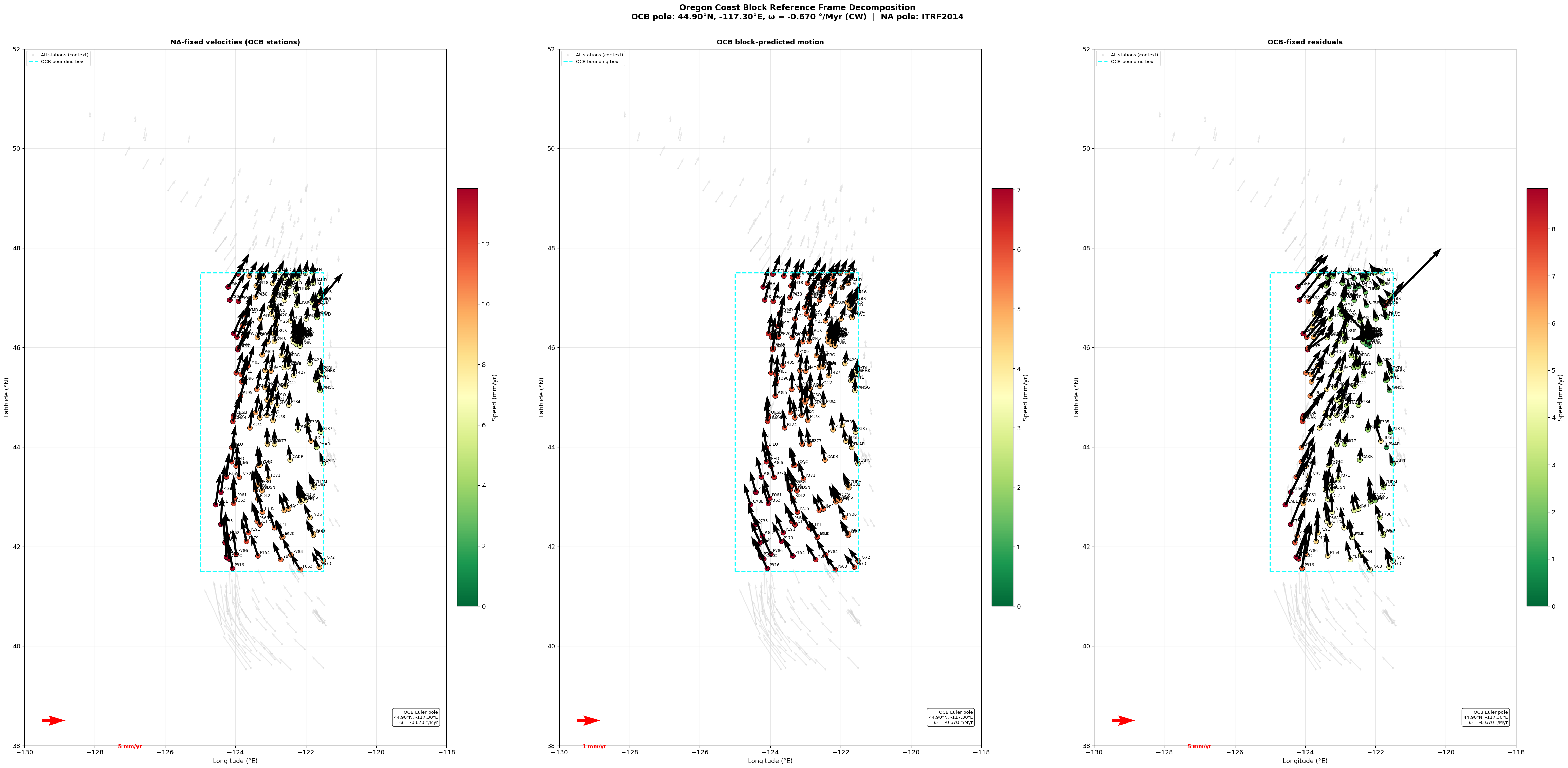
OCB-fixed velocity statistics — 179 stations inside OCB box:
  East  : +0.94 ± 2.72 mm/yr
  North : +3.36 ± 1.77 mm/yr
  Up    : -0.50 mm/yr

NA-fixed velocities at OCB stations (before correction):
  East  : +1.04 ± 3.63 mm/yr
  North : +8.44 ± 2.33 mm/yr

OCB-predicted rigid block motion (removed):
  East  : +0.10 ± 2.30 mm/yr
  North : +5.08 ± 0.74 mm/yr
15d. Network-Wide SSE Vector Offsets and Map#
For the 2015 slow slip event, we estimate 3-component (East, North, Up) offsets at all available stations using the step-function weighted least-squares method. The horizontal vectors are plotted as displacement arrows, providing a synoptic view of the slow slip spatial footprint. This pattern can be used to constrain slip distribution on the subduction interface.
# ══════════════════════════════════════════════════════════════════
# NETWORK-WIDE SSE OFFSET ESTIMATION — stations within 150 km of ALBH
# ══════════════════════════════════════════════════════════════════

ALBH_LAT = float(ds.sel(station='albh').lat)
ALBH_LON = float(ds.sel(station='albh').lon)
MAX_DIST_KM    = 150     # only process stations within this radius of ALBH
MIN_VALID_SSE  = 180     # minimum valid observations required
OFFSET_THRESH  = 20.0    # mm — discard any component offset larger than this
                          # (flags stations with data gaps or model failures
                          # straddling the SSE epoch)

def haversine_km(lat1, lon1, lat2, lon2):
    R = 6371.0
    dlat = np.radians(lat2 - lat1)
    dlon = np.radians(lon2 - lon1)
    a = (np.sin(dlat/2)**2
         + np.cos(np.radians(lat1)) * np.cos(np.radians(lat2)) * np.sin(dlon/2)**2)
    return R * 2 * np.arcsin(np.sqrt(a))

print(f"SSE offset estimation — stations within {MAX_DIST_KM} km of ALBH")
print(f"SSE step epoch : {SSE_EPOCH:.4f} ({SSE_TSTART})")
print(f"Offset threshold: ±{OFFSET_THRESH} mm\n")

sse_offsets = {}

for sname in station_list:
    stat_i = ds.sel(station=sname)
    lat_i  = float(stat_i.lat)
    lon_i  = float(stat_i.lon)

    if np.isnan(lat_i) or np.isnan(lon_i):
        continue

    dist_km = haversine_km(ALBH_LAT, ALBH_LON, lat_i, lon_i)
    if dist_km > MAX_DIST_KM:
        continue

    dec_yr_i = stat_i.dec_year.values
    e_i  = stat_i.east_m.values  * 1000
    n_i  = stat_i.north_m.values * 1000
    u_i  = stat_i.up_m.values    * 1000
    es_i = stat_i.east_sigma_m.values  * 1000
    ns_i = stat_i.north_sigma_m.values * 1000
    us_i = stat_i.up_sigma_m.values    * 1000

    if np.sum(~np.isnan(e_i)) < MIN_VALID_SSE:
        continue

    try:
        re = fit_model(dec_yr_i, e_i, sigma_mm=es_i, coseismic_times=all_steps)
        rn = fit_model(dec_yr_i, n_i, sigma_mm=ns_i, coseismic_times=all_steps)
        ru = fit_model(dec_yr_i, u_i, sigma_mm=us_i, coseismic_times=all_steps)

        e_off = re['params'][-1];  e_unc = re['param_std'][-1]
        n_off = rn['params'][-1];  n_unc = rn['param_std'][-1]
        u_off = ru['params'][-1];  u_unc = ru['param_std'][-1]

        # Discard station if any component exceeds the anomaly threshold
        if any(abs(v) > OFFSET_THRESH for v in [e_off, n_off, u_off]):
            print(f"  {sname.upper():6s}  REJECTED — offset exceeds ±{OFFSET_THRESH} mm "
                  f"(E={e_off:+.1f} N={n_off:+.1f} U={u_off:+.1f})")
            continue

        h_mag = np.sqrt(e_off**2 + n_off**2)
        h_snr = h_mag / np.sqrt(e_unc**2 + n_unc**2)

        sse_offsets[sname] = {
            'lat': lat_i, 'lon': lon_i, 'dist_km': dist_km,
            'Ve': e_off, 'Ve_sig': e_unc,
            'Vn': n_off, 'Vn_sig': n_unc,
            'Vu': u_off, 'Vu_sig': u_unc,
            'H_mag': h_mag, 'H_snr': h_snr,
        }
        print(f"  {sname.upper():6s}  dist={dist_km:5.1f} km  "
              f"E={e_off:+6.2f}±{e_unc:.2f}  "
              f"N={n_off:+6.2f}±{n_unc:.2f}  "
              f"U={u_off:+6.2f}±{u_unc:.2f} mm")

    except Exception as ex:
        print(f"  {sname.upper():6s}  FAILED: {ex}")

print(f"\nCompleted: {len(sse_offsets)} stations accepted within {MAX_DIST_KM} km of ALBH.")
sig_stations = {s: v for s, v in sse_offsets.items() if v['H_snr'] >= 2.0}
print(f"Stations with H_SNR ≥ 2.0: {len(sig_stations)}")
SSE offset estimation — stations within 150 km of ALBH
SSE step epoch : 2015.9890 (2015-12-28)
Offset threshold: ±20.0 mm

  ALBH    dist=  0.0 km  E= -2.75±0.14  N= -0.19±0.10  U= -1.40±0.30 mm
  ARLI    dist=102.4 km  E= -0.90±0.11  N= +0.45±0.10  U= +0.37±0.39 mm
  BAMF    dist=130.9 km  E= -2.40±0.16  N= -0.76±0.15  U= +2.63±0.39 mm
  BELI    dist= 84.6 km  E= -0.29±0.12  N= +1.77±0.13  U= -2.36±0.37 mm
  BILS    dist=110.4 km  E= -1.26±0.25  N= -2.44±0.24  U= -1.18±0.50 mm
  BLYN    REJECTED — offset exceeds ±20.0 mm (E=+7.0 N=-8.9 U=+121.1)
  BRN3    dist=103.8 km  E= -0.33±0.13  N= -0.05±0.14  U= +1.28±0.54 mm
  CHCM    dist= 67.5 km  E= -0.48±0.13  N= +0.10±0.10  U= -1.82±0.29 mm
  CHLW    REJECTED — offset exceeds ±20.0 mm (E=+4991.8 N=+4055.7 U=+264.8)
  CHWK    dist=137.9 km  E= -0.79±0.13  N= -0.20±0.10  U= -1.06±0.40 mm
  CLRS    dist= 67.3 km  E= -1.30±0.15  N= +0.91±0.10  U= +2.17±0.32 mm
  CNCR    dist=129.2 km  E= -0.55±0.11  N= +1.66±0.15  U= -1.39±0.54 mm
  COUP    dist= 62.3 km  E= -1.82±0.19  N= -0.44±0.14  U= -0.88±0.34 mm
  CSKI    dist=146.0 km  E= -0.89±0.12  N= -0.32±0.09  U= -2.27±0.29 mm
  CULM    REJECTED — offset exceeds ±20.0 mm (E=+5411.0 N=+4504.9 U=+655.3)
  CUSH    dist=109.3 km  E= -0.97±0.14  N= -0.74±0.12  U= +0.05±0.46 mm
  DEEJ    dist=107.5 km  E= -0.63±0.16  N= -0.96±0.23  U= +0.25±0.47 mm
  ELSR    dist=113.0 km  E= -2.05±0.17  N= -1.03±0.09  U= -2.40±0.30 mm
  JOBO    dist= 79.8 km  E= -0.95±0.12  N= -0.73±0.11  U= -2.77±0.38 mm
  KTBW    dist=106.9 km  E= -1.19±0.14  N= -1.00±0.17  U= -0.69±0.28 mm
  LKCP    dist=132.5 km  E= -0.79±0.12  N= -0.50±0.10  U= -0.09±0.33 mm
  LNGB    dist=141.1 km  E= -1.42±0.13  N= +0.26±0.09  U= -2.65±0.29 mm
  MKAH    dist= 81.4 km  E= -1.67±0.13  N= -0.28±0.12  U= +3.61±0.37 mm
  MRIB    REJECTED — offset exceeds ±20.0 mm (E=+4587.1 N=+4518.7 U=-945.9)
  NANO    dist=109.8 km  E= -0.19±0.12  N= -0.31±0.11  U= -0.22±0.29 mm
  NEAH    dist= 84.7 km  E= -1.27±0.16  N= -0.38±0.14  U= -1.28±0.50 mm
  OYLR    dist=139.6 km  E= -0.92±0.16  N= -0.21±0.11  U= -0.24±0.30 mm
  P064    dist= 46.7 km  E= +0.19±0.14  N= -0.66±0.15  U= -0.60±0.33 mm
  P399    dist=106.7 km  E= -1.84±0.23  N= -0.50±0.20  U= +1.78±0.56 mm
  P400    dist=100.4 km  E= -0.40±0.15  N= -0.53±0.16  U= +2.12±0.51 mm
  P401    dist= 93.9 km  E= -0.52±0.09  N= +0.39±0.09  U= +0.02±0.24 mm
  P402    dist= 92.2 km  E= -0.41±0.09  N= +0.01±0.09  U= -1.69±0.26 mm
  P403    dist= 60.6 km  E= -1.24±0.18  N= -1.13±0.18  U= +1.13±0.42 mm
  P418    dist=128.4 km  E= -1.62±0.12  N= +0.53±0.10  U= +1.28±0.29 mm
  P419    dist=109.4 km  E= +0.57±0.16  N= +1.28±0.14  U= -3.48±0.39 mm
  P423    dist=129.1 km  E= -2.05±0.12  N= -1.11±0.11  U= -1.45±0.32 mm
  P424    dist= 77.7 km  E= -1.09±0.14  N= -1.17±0.12  U= -1.51±0.32 mm
  P426    dist= 97.4 km  E= +0.62±0.27  N= -1.18±0.20  U= -0.19±0.67 mm
  P435    dist= 36.7 km  E= -0.79±0.13  N= -0.81±0.16  U= -1.40±0.35 mm
  P436    dist= 46.4 km  E= -0.58±0.12  N= +0.51±0.10  U= -0.71±0.31 mm
  P437    dist= 87.6 km  E= -1.27±0.13  N= -0.36±0.11  U= -1.75±0.30 mm
  P438    dist= 60.4 km  E= +0.47±0.22  N= +0.51±0.15  U= +1.17±0.43 mm
  P439    dist= 55.4 km  E= -1.83±0.12  N= -1.13±0.11  U= -0.59±0.26 mm
  P440    dist= 89.6 km  E= -0.03±0.13  N= +0.08±0.12  U= +1.65±0.38 mm
  P441    dist=115.0 km  E= +0.02±0.13  N= -0.24±0.14  U= -0.83±0.43 mm
  P442    dist=139.1 km  E= -0.93±0.11  N= -0.16±0.12  U= +1.13±0.36 mm
  P815    dist= 94.0 km  E= -0.01±0.08  N= -0.13±0.07  U= -0.07±0.25 mm
  P816    dist= 94.0 km  E= -0.61±0.08  N= -0.43±0.07  U= +0.20±0.25 mm
  PABH    dist=141.4 km  E= -0.78±0.10  N= +0.34±0.08  U= +0.45±0.26 mm
  PFLD    dist=104.8 km  E= -0.37±0.15  N= -0.19±0.09  U= +3.40±0.36 mm
  PGC5    dist= 28.9 km  E= -2.17±0.18  N= -0.49±0.12  U= -2.34±0.33 mm
  PRDY    dist=128.9 km  E= -1.76±0.12  N= +0.31±0.09  U= -3.18±0.29 mm
  PTAA    dist= 30.4 km  E= -1.11±0.16  N= +0.47±0.15  U= -3.70±0.40 mm
  PTAL    dist=139.3 km  E= -0.98±0.12  N= +0.33±0.11  U= +0.03±0.30 mm
  PTRF    dist= 70.4 km  E= -5.90±0.17  N= +3.80±0.14  U= -6.68±0.41 mm
  PUPU    dist=148.1 km  E= -0.23±0.23  N= -1.73±0.22  U= -2.41±0.66 mm
  RPT5    dist=138.9 km  E= -1.35±0.13  N= +0.30±0.09  U= -1.41±0.30 mm
  SAMM    dist=143.7 km  E= -0.76±0.18  N= -1.98±0.18  U= -2.96±0.41 mm
  SC02    dist= 39.4 km  E= -0.76±0.17  N= +0.17±0.11  U= -1.82±0.28 mm
  SC03    dist= 65.8 km  E= -0.53±0.19  N= -0.47±0.21  U= -1.04±0.36 mm
  SC04    dist= 61.4 km  E= -0.80±0.13  N= -0.93±0.12  U= -0.61±0.31 mm
  SEAT    dist=119.9 km  E= -1.30±0.13  N= +0.26±0.10  U= -2.04±0.32 mm
  SEDR    dist= 94.3 km  E= -0.94±0.13  N= -0.41±0.09  U= +0.11±0.34 mm
  SEQM    dist= 43.2 km  E= -1.67±0.14  N= -0.46±0.12  U= -1.87±0.37 mm
  SKGT    REJECTED — offset exceeds ±20.0 mm (E=+4927.2 N=+4301.6 U=+1041.2)
  SMAI    dist=128.5 km  E= -0.56±0.14  N= -0.09±0.11  U= -2.98±0.32 mm
  SSHO    dist=117.4 km  E= -1.35±0.15  N= -0.80±0.10  U= -2.01±0.33 mm
  TACO    dist=149.7 km  E= -1.43±0.12  N= +1.09±0.11  U= +0.56±0.36 mm
  UFDA    dist= 93.2 km  E= -1.49±0.16  N= +0.64±0.11  U= -4.52±0.33 mm
  WHD5    dist= 59.1 km  E= -2.79±0.22  N= -0.14±0.15  U= -1.50±0.30 mm

Completed: 65 stations accepted within 150 km of ALBH.
Stations with H_SNR ≥ 2.0: 61
# ══════════════════════════════════════════════════════════════════
# WRITE SSE OFFSET TEXT FILE
# ══════════════════════════════════════════════════════════════════

sse_filename = "gnss_SSE_offsets_2015.txt"

with open(sse_filename, 'w') as f:
    f.write("# GNSS 2015 Slow Slip Event Offsets\n")
    f.write(f"# Event window  : {SSE_TSTART} → {SSE_TEND}\n")
    f.write(f"# SSE epoch     : {SSE_EPOCH:.4f}\n")
    f.write(f"# Station radius: {MAX_DIST_KM} km of ALBH "
            f"({ALBH_LAT:.3f}°N, {ALBH_LON:.3f}°E)\n")
    f.write(f"# Offset threshold: ±{OFFSET_THRESH} mm (anomalous stations excluded)\n")
    f.write("# Method: weighted least-squares step function fit\n")
    f.write("# All offsets in mm; uncertainties are 1-sigma formal errors\n")
    f.write("#\n")
    f.write(f"# {'station':<8} {'lat':>9} {'lon':>10} {'dist_km':>9} "
            f"{'Ve':>9} {'Ve_sig':>8} "
            f"{'Vn':>9} {'Vn_sig':>8} "
            f"{'Vu':>9} {'Vu_sig':>8} "
            f"{'H_mag':>8} {'H_snr':>7}\n")
    f.write("# " + "-"*105 + "\n")

    for sname, v in sorted(sse_offsets.items(), key=lambda x: x[1]['dist_km']):
        f.write(f"  {sname:<8} {v['lat']:9.4f} {v['lon']:10.4f} {v['dist_km']:9.1f} "
                f"{v['Ve']:+9.4f} {v['Ve_sig']:8.4f} "
                f"{v['Vn']:+9.4f} {v['Vn_sig']:8.4f} "
                f"{v['Vu']:+9.4f} {v['Vu_sig']:8.4f} "
                f"{v['H_mag']:8.4f} {v['H_snr']:7.2f}\n")

print(f"Wrote {len(sse_offsets)} station offsets to '{sse_filename}'")
print(f"(sorted by distance from ALBH)")
Wrote 65 station offsets to 'gnss_SSE_offsets_2015.txt'
(sorted by distance from ALBH)
# ══════════════════════════════════════════════════════════════════
# SSE VECTOR MAP — stations within 150 km of ALBH
# ══════════════════════════════════════════════════════════════════

s_lats  = np.array([v['lat']    for v in sse_offsets.values()])
s_lons  = np.array([v['lon']    for v in sse_offsets.values()])
s_ve    = np.array([v['Ve']     for v in sse_offsets.values()])
s_vn    = np.array([v['Vn']     for v in sse_offsets.values()])
s_vu    = np.array([v['Vu']     for v in sse_offsets.values()])
s_hmag  = np.array([v['H_mag']  for v in sse_offsets.values()])
s_hsnr  = np.array([v['H_snr']  for v in sse_offsets.values()])
s_names = list(sse_offsets.keys())

fig, axes = plt.subplots(1, 2, figsize=(14, 7))

for ax, (vals, cmap, clabel, title) in zip(axes, [
    (s_hmag, 'hot_r',  'Horizontal SSE offset (mm)', 'Horizontal Displacement Vectors'),
    (s_vu,   'RdBu',   'Vertical SSE offset (mm)',   'Vertical Displacement'),
]):
    vmax = np.percentile(np.abs(vals), 97) if len(vals) > 0 else 1.0
    vmin = -vmax if cmap == 'RdBu' else 0

    sc = ax.scatter(s_lons, s_lats, c=vals, cmap=cmap,
                    vmin=vmin, vmax=vmax,
                    s=60, edgecolors='k', linewidths=0.5, zorder=4)
    fig.colorbar(sc, ax=ax, shrink=0.8).set_label(clabel)

    # Draw a circle showing the 150 km search radius around ALBH
    theta = np.linspace(0, 2*np.pi, 360)
    dlat  = (MAX_DIST_KM / 111.0)
    dlon  = (MAX_DIST_KM / (111.0 * np.cos(np.radians(ALBH_LAT))))
    ax.plot(ALBH_LON + dlon*np.cos(theta),
            ALBH_LAT + dlat*np.sin(theta),
            'k--', lw=0.8, alpha=0.4, label=f'{MAX_DIST_KM} km radius')

    # Station labels
    for sname, lon_s, lat_s in zip(s_names, s_lons, s_lats):
        ax.annotate(sname.upper(), (lon_s, lat_s),
                    xytext=(4, 4), textcoords='offset points', fontsize=7)

    # Horizontal vectors on left panel only
    if cmap == 'hot_r':
        mask_sig = s_hsnr >= 1.5
        if mask_sig.sum() > 0:
            ax.quiver(s_lons[mask_sig], s_lats[mask_sig],
                      s_ve[mask_sig], s_vn[mask_sig],
                      scale=None, scale_units='xy', angles='xy',
                      width=0.004, color='k', zorder=5)
        # Reference arrow
        ref_lon = s_lons.min() + 0.1
        ref_lat = s_lats.min() + 0.1
        ax.quiver(ref_lon, ref_lat, 2, 0,
                  scale=None, scale_units='xy', angles='xy',
                  width=0.005, color='k', zorder=6)
        ax.text(ref_lon + 1.0, ref_lat - 0.15, '2 mm', fontsize=8, ha='center')

    # Mark ALBH
    ax.scatter(ALBH_LON, ALBH_LAT, s=150, c='cyan', marker='*',
               edgecolors='k', linewidths=0.8, zorder=7, label='ALBH')

    ax.set_xlabel("Longitude (°E)")
    ax.set_ylabel("Latitude (°N)")
    ax.set_title(f"2015 SSE — {title}\n"
                 f"({len(sse_offsets)} stations within {MAX_DIST_KM} km of ALBH, "
                 f"threshold ±{OFFSET_THRESH} mm)")
    ax.set_aspect('equal', adjustable='box')
    ax.legend(fontsize=8, loc='upper right')
    ax.grid(True, alpha=0.3)

plt.suptitle("2015 Cascadia ETS Displacement Field", fontsize=13)
plt.tight_layout()
plt.show()
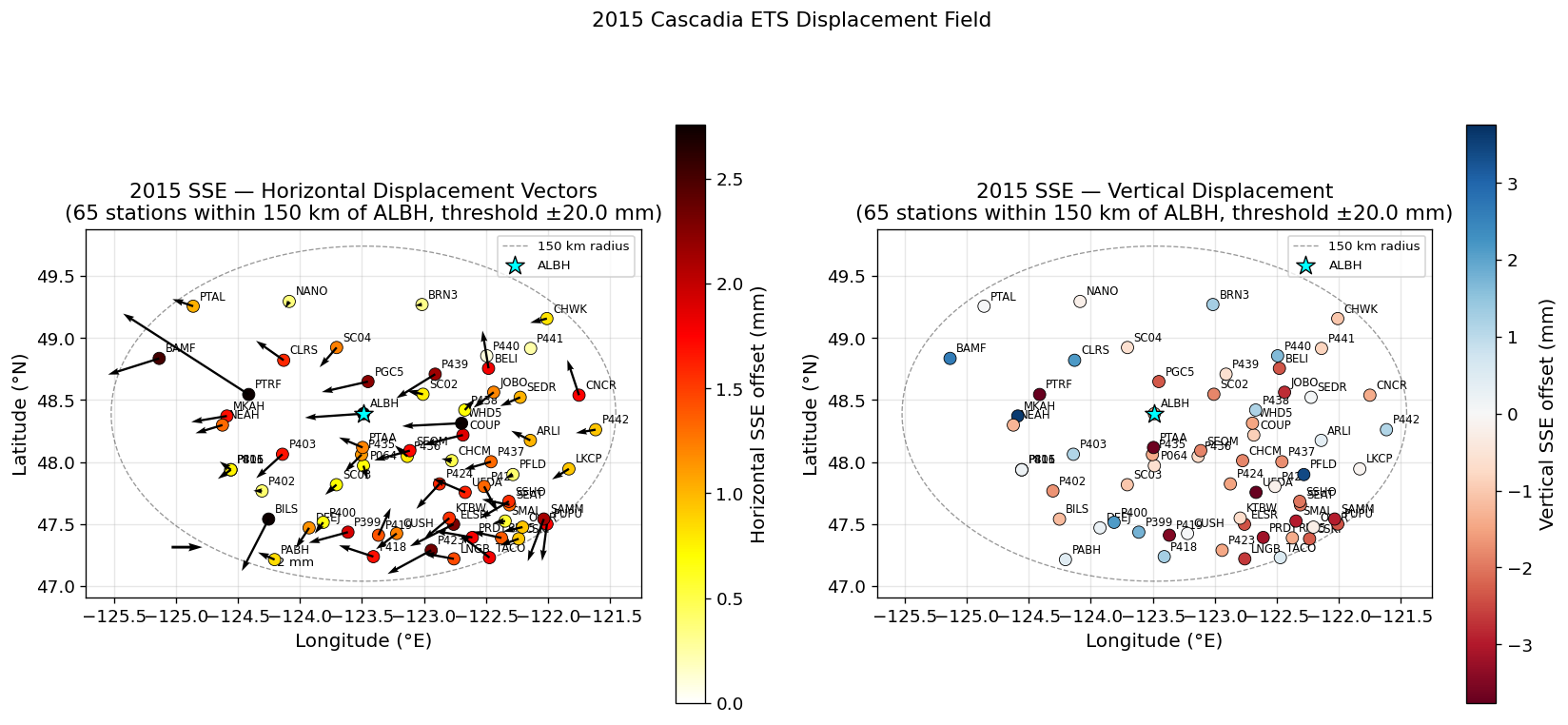
# ══════════════════════════════════════════════════════════════════
# SSE ALONG-STRIKE PROFILE
# Shows how SSE offset magnitude varies along the subduction zone
# ══════════════════════════════════════════════════════════════════

# Project onto a rough along-strike axis for Cascadia (~N30°W = azimuth 330°)
# Strike-perpendicular = trench-normal direction (NE)
STRIKE_AZ = 330.0   # degrees clockwise from North

def project_along_strike(lats, lons, az_deg, origin_lat=47.0, origin_lon=-123.5):
    """Project lat/lon onto along-strike and across-strike distances (km)."""
    R = 6371.0
    dlat = np.radians(lats - origin_lat)
    dlon = np.radians(lons - origin_lon)
    lat_r = np.radians(lats)

    # Local Cartesian (km)
    dx = R * dlon * np.cos(np.radians(origin_lat))
    dy = R * dlat

    # Rotate to along-strike / across-strike
    az_r = np.radians(az_deg)
    along  = -dx * np.sin(az_r) + dy * np.cos(az_r)
    across =  dx * np.cos(az_r) + dy * np.sin(az_r)
    return along, across

along, across = project_along_strike(s_lats, s_lons, STRIKE_AZ)

fig, axes = plt.subplots(1, 2, figsize=(13, 5))

for ax, dist, xlabel in [(axes[0], along, 'Along-strike distance (km)'),
                          (axes[1], across, 'Across-strike distance (km)')]:
    ax.scatter(dist, s_hmag, c=s_hmag, cmap='hot_r', s=20, alpha=0.6, zorder=3)

    # Error bars for significant detections
    mask_p = s_hsnr >= 1.5
    if mask_p.sum() > 0:
        e_unc_plot = np.sqrt(
            np.array([v['Ve_sig'] for v in sse_offsets.values()])**2 +
            np.array([v['Vn_sig'] for v in sse_offsets.values()])**2
        )
        ax.errorbar(dist[mask_p], s_hmag[mask_p],
                    yerr=2*e_unc_plot[mask_p],
                    fmt='none', ecolor='gray', elinewidth=0.5, capsize=2, alpha=0.5)

    ax.set_xlabel(xlabel)
    ax.set_ylabel("Horizontal SSE offset (mm)")
    ax.grid(True, alpha=0.3)

axes[0].set_title("SSE Offset vs Along-Strike Position")
axes[1].set_title("SSE Offset vs Across-Strike Position\n(negative = toward trench)")

plt.suptitle("2015 Cascadia SSE — Spatial Profile", fontsize=13)
plt.tight_layout()
plt.show()
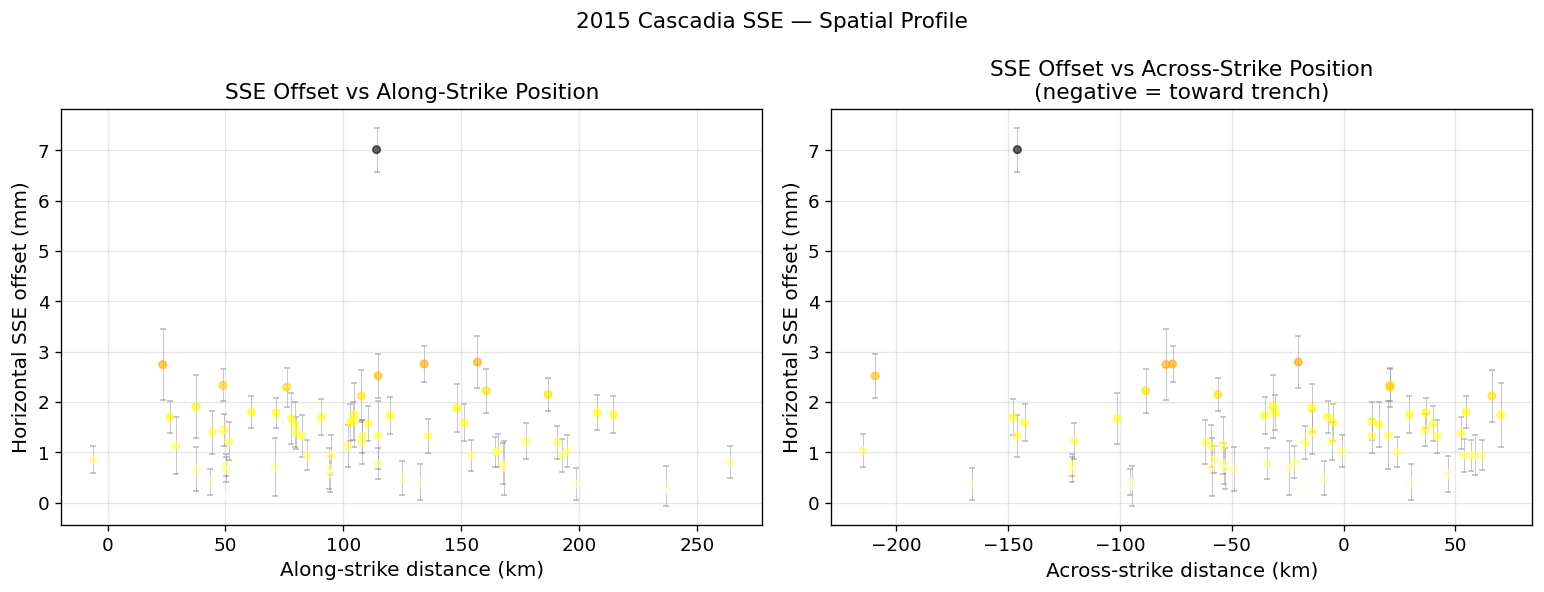
16. Power Spectrum and Noise Characteristics of Daily Position Time Series#
GPS/GNSS daily position time series are not white noise. The residuals after removing the deterministic model (trend, seasonal, coseismic) contain a characteristic colored-noise signature whose spectral structure controls how measurement uncertainties scale with averaging time and, ultimately, how precisely transient signals can be detected.
Noise taxonomy in GPS time series#
Noise type |
Spectral index α |
PSD shape |
Physical origin |
|---|---|---|---|
White noise |
0 |
flat |
Daily measurement noise (thermal, multipath) |
Flicker noise |
−1 |
1/f |
Monument instability, atmospheric loading |
Random walk |
−2 |
1/f² |
Slow monument motion, hydrological loading |
The one-sided power spectral density (PSD) of a stationary noise process follows:
where the spectral index \(\alpha\) determines whether uncertainties grow (\(\alpha > 0\)) or remain bounded (\(\alpha = 0\)) as the averaging period increases. For GPS, the dominant contributors are typically white noise + flicker noise, though random-walk components are detectable at many monuments.
We characterize the residual noise using three complementary techniques:
Lomb-Scargle / FFT periodogram — resolves spectral peaks at annual, semi-annual, and sub-seasonal periods and reveals the broadband colored-noise floor
Spectral index fitting — fits a power-law slope to the broadband PSD to classify noise type
Allan Deviation (ADEV) — a time-domain estimator of noise as a function of averaging time, complementary to the frequency-domain view and robust to non-stationarity
from scipy.signal import periodogram, welch
from scipy.stats import linregress

# ── Prepare residuals for spectral analysis ───────────────────────────────
# Use the ALBH East residuals (longest, cleanest record)
east_res = results['east_mm']['residuals'].copy()
valid_mask = ~np.isnan(east_res)
t_full = df_albh.dec_year.values

# Interpolate over NaN gaps — but only within the valid range to avoid
# extrapolation at the edges, which can produce NaN or Inf.
t_valid = t_full[valid_mask]
d_valid = east_res[valid_mask]

# Restrict the uniform grid to the span of valid data
t_uniform = t_full[(t_full >= t_valid[0]) & (t_full <= t_valid[-1])]
east_interp = np.interp(t_uniform, t_valid, d_valid)

# Final safety check: drop any residual non-finite values
finite_mask = np.isfinite(east_interp)
east_interp = east_interp[finite_mask]

# Sampling frequency: 1 sample/day
fs = 1.0   # cycles per day

# ── Welch PSD (better variance than raw periodogram) ─────────────────────
nperseg = min(512, len(east_interp) // 4)
f_welch, psd_welch = welch(east_interp, fs=fs, nperseg=nperseg,
                            window='hann', detrend='linear', scaling='density')

# Skip the DC bin
f_welch = f_welch[1:]; psd_welch = psd_welch[1:]

# Convert to cycles/year for readability
f_cpy = f_welch * 365.25    # cycles per year

# ── Lomb-Scargle periodogram on the original (possibly gapped) residuals ─
from scipy.signal import lombscargle

d_ls = d_valid - np.nanmean(d_valid)   # zero-mean

# Frequency grid: 0.5 to 180 cycles/yr
f_ls_cpy = np.logspace(np.log10(0.5), np.log10(180), 3000)
f_ls_rad = f_ls_cpy * 2 * np.pi / 365.25

pgram_ls = lombscargle(t_valid * 365.25, d_ls, f_ls_rad, normalize=False)
pgram_ls_psd = pgram_ls / (np.diff(f_ls_cpy)[0] * len(d_ls))

print(f"Spectral analysis of ALBH East residuals")
print(f"  N valid points : {valid_mask.sum()}")
print(f"  Record length  : {t_valid[-1] - t_valid[0]:.1f} yr")
print(f"  Uniform grid   : {len(east_interp)} points (clipped to valid span)")
print(f"  Welch nperseg  : {nperseg}  (frequency resolution = {fs/nperseg * 365.25:.3f} cpy)")
Spectral analysis of ALBH East residuals
  N valid points : 5833
  Record length  : 16.0 yr
  Uniform grid   : 5833 points (clipped to valid span)
  Welch nperseg  : 512  (frequency resolution = 0.713 cpy)
# ── Fit spectral index (power-law slope) to broadband PSD ───────────────
# Use Welch PSD in log-log space; fit between 5 and 90 cpyr to avoid
# annual/semi-annual peaks and Nyquist roll-off

mask_fit = (f_cpy >= 5.0) & (f_cpy <= 90.0)
log_f   = np.log10(f_cpy[mask_fit])
log_psd = np.log10(psd_welch[mask_fit])

slope, intercept, r_val, _, _ = linregress(log_f, log_psd)
alpha = -slope    # PSD ∝ f^slope → noise spectral index α = −slope

print(f"Power-law fit (5–90 cpy):")
print(f"  Spectral slope  = {slope:+.3f}")
print(f"  Noise index α   = {alpha:.3f}")
print(f"  R²              = {r_val**2:.3f}")
print()
if alpha < 0.3:
    noise_type = "predominantly white"
elif alpha < 0.7:
    noise_type = "transitional white/flicker"
elif alpha < 1.4:
    noise_type = "predominantly flicker (1/f)"
elif alpha < 1.8:
    noise_type = "transitional flicker/random-walk"
else:
    noise_type = "predominantly random walk"
print(f"  Noise character : {noise_type}  (α ≈ {alpha:.2f})")

# ── 3-component spectral index comparison ───────────────────────────────
def safe_interp(res_array, t_array):
    """Interpolate residuals onto uniform grid, clipped to valid span."""
    valid = np.isfinite(res_array)
    t_v = t_array[valid]
    d_v = res_array[valid]
    t_uniform = t_array[(t_array >= t_v[0]) & (t_array <= t_v[-1])]
    interped = np.interp(t_uniform, t_v, d_v)
    return interped[np.isfinite(interped)]

print()
print(f"{'Component':<10} {'α':>8} {'Noise type'}")
print("-" * 48)
alpha_dict = {}
for comp, label, color in comp_info:
    res_c = results[comp]['residuals'].copy()
    t_c   = df_albh.dec_year.values
    res_interp_c = safe_interp(res_c, t_c)
    f_c, psd_c = welch(res_interp_c, fs=1.0, nperseg=nperseg,
                       window='hann', detrend='linear', scaling='density')
    f_c = f_c[1:]; psd_c = psd_c[1:]
    f_cpy_c = f_c * 365.25
    mk = (f_cpy_c >= 5.0) & (f_cpy_c <= 90.0)
    sl, ic, rv, _, _ = linregress(np.log10(f_cpy_c[mk]), np.log10(psd_c[mk]))
    a = -sl
    alpha_dict[comp] = (a, f_cpy_c, psd_c)
    if a < 0.5:
        nt = "white-dominated"
    elif a < 1.4:
        nt = "flicker-dominated"
    else:
        nt = "random-walk-dominated"
    print(f"  {label:<10} {a:>6.3f}   {nt}")
Power-law fit (5–90 cpy):
  Spectral slope  = -0.843
  Noise index α   = 0.843
  R²              = 0.833

  Noise character : predominantly flicker (1/f)  (α ≈ 0.84)

Component         α Noise type
------------------------------------------------
  East        0.843   flicker-dominated
  North       0.803   flicker-dominated
  Up          0.669   flicker-dominated
# ── Spectral plot — 3 components + reference slopes ─────────────────────
fig, axes = plt.subplots(1, 3, figsize=(16, 5))

ref_f  = np.array([1.0, 100.0])   # cpy
slope_labels = [
    (0,  'k-',   'White (α=0)',       1.0),
    (-1, 'k--',  'Flicker (α=1)',     1.0),
    (-2, 'k:',   'Random walk (α=2)', 1.0),
]

for ax, (comp, label, color) in zip(axes, comp_info):
    a, f_cpy_c, psd_c = alpha_dict[comp]

    ax.loglog(f_cpy_c, psd_c, color=color, lw=1.2, alpha=0.9, label='Welch PSD')

    # Mark annual and semi-annual peaks
    for p_cpy, ptxt in [(1.0, 'annual'), (2.0, 'semi-ann'), (4.0, 'qtr-ann')]:
        ax.axvline(p_cpy, color='gray', lw=0.8, ls='--', alpha=0.6)
        ax.text(p_cpy * 1.07, ax.get_ylim()[0] if ax.get_ylim()[0] != 0 else 1e-4,
                ptxt, fontsize=7, color='gray', rotation=90, va='bottom',
                transform=ax.get_xaxis_transform())

    # Reference power-law slopes (anchored at 10 cpy)
    anchor_f = 10.0
    anchor_psd = float(10**np.interp(np.log10(anchor_f),
                                     np.log10(f_cpy_c), np.log10(psd_c)))
    for sl, ls, slabel, scale in slope_labels:
        ref_psd = anchor_psd * scale * (ref_f / anchor_f)**sl
        ax.loglog(ref_f, ref_psd, ls, lw=1.0, alpha=0.6, label=slabel)

    # Best-fit slope line
    mask_f = (f_cpy_c >= 5) & (f_cpy_c <= 90)
    sl_line = np.log10(anchor_psd) + (-a) * (np.log10(f_cpy_c[mask_f]) - np.log10(anchor_f))
    ax.loglog(f_cpy_c[mask_f], 10**sl_line, color=color, lw=2.0, ls='-.',
              alpha=0.8, label=f'Fit α={a:.2f}')

    ax.set_xlabel("Frequency (cycles yr⁻¹)")
    ax.set_ylabel("PSD (mm² cpyr⁻¹)")
    ax.set_title(f"ALBH {label} — Power Spectrum")
    ax.set_xlim(0.3, 180)
    ax.legend(fontsize=8, loc='upper right')
    ax.grid(True, which='both', alpha=0.3)

plt.suptitle("ALBH Residual Power Spectral Density — All Components", fontsize=13)
plt.tight_layout()
plt.show()
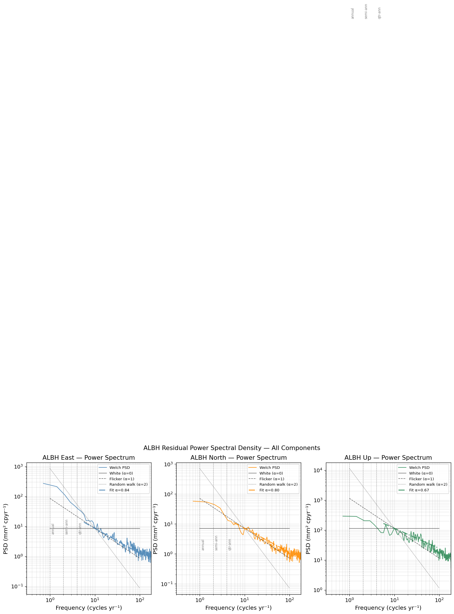
# ── Lomb-Scargle periodogram — spectral peak identification ─────────────
# Identify statistically significant peaks (signal-to-noise > threshold)

fig, axes = plt.subplots(3, 1, figsize=(14, 10), sharex=True)
comp_info_ls = [
    ('east_mm',  'East',  'steelblue'),
    ('north_mm', 'North', 'darkorange'),
    ('up_mm',    'Up',    'seagreen'),
]

PEAK_SNR_THRESH = 5.0    # peak must exceed 5× local median PSD to be labeled

for ax, (comp, label, color) in zip(axes, comp_info_ls):
    res_c = results[comp]['residuals'].copy()
    valid_c = ~np.isnan(res_c)
    d_ls = res_c[valid_c] - np.nanmean(res_c[valid_c])
    t_ls = df_albh.dec_year.values[valid_c] * 365.25   # in days

    f_ls_cpy_c = np.linspace(0.2, 100, 5000)
    f_ls_rad_c = f_ls_cpy_c * 2 * np.pi / 365.25
    pgram_c = lombscargle(t_ls, d_ls, f_ls_rad_c, normalize=True)

    ax.semilogy(f_ls_cpy_c, pgram_c, color=color, lw=0.8, alpha=0.85, label='L-S power')

    # False alarm level (0.1% FAP via exponential approx)
    N_eff = len(d_ls)
    fap_level = 1.0 - (0.001) ** (1.0 / N_eff)
    ax.axhline(fap_level, color='red', lw=1.0, ls='--', alpha=0.7,
               label=f'0.1% FAP ({fap_level:.4f})')

    # Mark known geophysical frequencies
    known = [(1.0, 'Annual'), (2.0, 'Semi-ann'), (3.0, 'Tri-ann'), (4.0, 'Qtr-ann')]
    for f0, fname in known:
        ax.axvline(f0, color='k', lw=0.7, ls=':', alpha=0.5)
        ax.text(f0 + 0.05, ax.get_ylim()[1] * 0.7 if ax.get_ylim()[1] != 0 else 0.5,
                fname, fontsize=7.5, color='k', rotation=90,
                transform=ax.get_xaxis_transform(), va='top')

    ax.set_ylabel(f"{label} — L-S Power")
    ax.legend(fontsize=8, loc='upper right')
    ax.grid(True, which='both', alpha=0.25)
    ax.set_xlim(0.2, 100)

axes[0].set_title("ALBH Residuals — Lomb-Scargle Periodogram\n"
                   "(seasonal signals already removed from model; residual peaks = unmodeled periodicities)")
axes[-1].set_xlabel("Frequency (cycles yr⁻¹)")
plt.tight_layout()
plt.show()

# ── Print dominant residual peaks ─────────────────────────────────────────
print("Dominant spectral peaks in ALBH East residuals:")
print(f"{'Period (yr)':<14} {'Freq (cpy)':<13} {'Period (days)':<16} {'L-S Power'}")
print("-" * 58)
res_east_c = results['east_mm']['residuals'].copy()
valid_e = ~np.isnan(res_east_c)
d_pk = res_east_c[valid_e] - np.nanmean(res_east_c[valid_e])
t_pk = df_albh.dec_year.values[valid_e] * 365.25
f_pk = np.linspace(0.3, 90, 8000)
f_pk_rad = f_pk * 2 * np.pi / 365.25
pgram_pk = lombscargle(t_pk, d_pk, f_pk_rad, normalize=True)
# Local maxima above FAP
from scipy.signal import argrelmax
peaks = argrelmax(pgram_pk, order=10)[0]
peaks_sig = peaks[pgram_pk[peaks] > fap_level]
peaks_sorted = peaks_sig[np.argsort(pgram_pk[peaks_sig])[::-1]]
for pidx in peaks_sorted[:10]:
    fp = f_pk[pidx]
    print(f"  {1/fp:<14.4f} {fp:<13.4f} {365.25/fp:<16.1f} {pgram_pk[pidx]:.4f}")
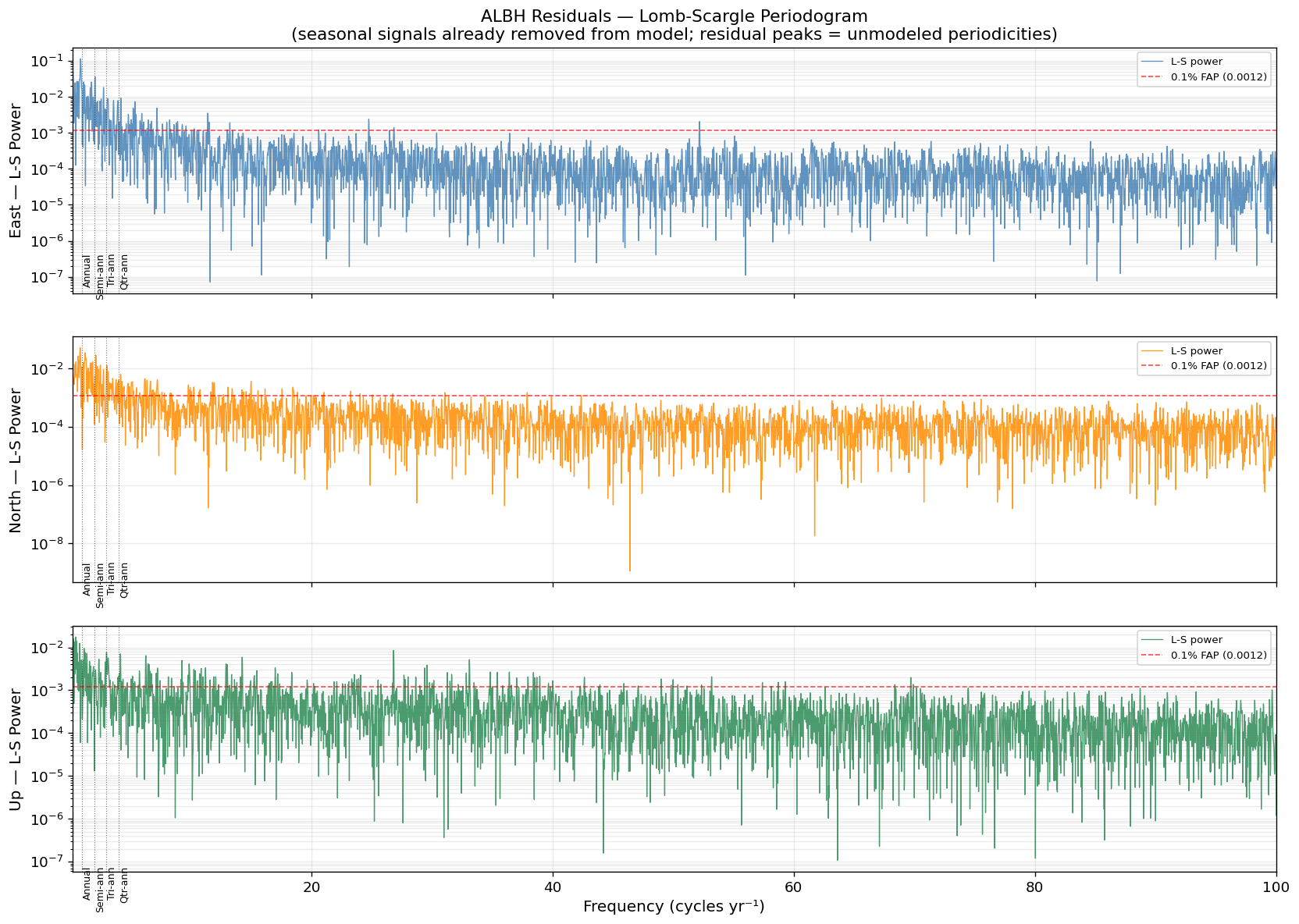
Dominant spectral peaks in ALBH East residuals:
Period (yr)    Freq (cpy)    Period (days)    L-S Power
----------------------------------------------------------
  1.1772         0.8495        430.0            0.1148
  0.4880         2.0494        178.2            0.0368
  0.9030         1.1074        329.8            0.0292
  1.5713         0.6364        573.9            0.0269
  0.5689         1.7578        207.8            0.0258
  2.6420         0.3785        965.0            0.0243
  0.3629         2.7558        132.5            0.0183
  0.7324         1.3653        267.5            0.0107
  0.3898         2.5652        142.4            0.0094
  0.2386         4.1912        87.1             0.0092
# ── Allan Deviation: time-domain noise characterization ─────────────────
# ADEV(τ) = sqrt[ 0.5 * <(x̄_{k+1} - x̄_k)²> ] where x̄_k are non-overlapping
# block means of length τ.
# Slope in log-log space: ADEV ∝ τ^H where H = (1-α)/2 for power-law noise.
# White:   H = -½  → ADEV ∝ 1/√τ
# Flicker: H =  0  → ADEV ∝ const
# RW:      H = +½  → ADEV ∝ √τ

def allan_deviation(x, tau_max_days=None):
    x = np.asarray(x, dtype=float)
    n = len(x)
    if tau_max_days is None:
        tau_max_days = n // 4
    taus, adevs = [], []
    for tau in range(1, min(tau_max_days + 1, n // 4)):
        n_blocks = n // tau
        if n_blocks < 4:
            break
        blocks = x[:n_blocks * tau].reshape(n_blocks, tau)
        block_means = np.nanmean(blocks, axis=1)
        diffs = np.diff(block_means)
        adev = np.sqrt(0.5 * np.nanmean(diffs**2))
        taus.append(tau)
        adevs.append(adev)
    return np.array(taus), np.array(adevs)


# ── Reference ADEV slopes ─────────────────────────────────────────────────
def adev_white(tau, sigma0):
    return sigma0 / np.sqrt(tau)

def adev_flicker(tau, sigma_f):
    return sigma_f * np.ones_like(tau, dtype=float)

def adev_rw(tau, sigma_rw):
    return sigma_rw * np.sqrt(tau)

# ── Fit combined noise model to ALBH East ────────────────────────────────
pre_sse = df_albh.time < t_event_start
pre_res_e = results['east_mm']['residuals'][pre_sse].copy()
pre_res_e = pre_res_e[~np.isnan(pre_res_e)]

taus_e, adevs_e = allan_deviation(pre_res_e, tau_max_days=400)

# Three-component noise model: white + flicker + random walk
# ADEV² ≈ σ_w² / τ + σ_f² + σ_rw² * τ
def adev_model(tau, sw, sf, srw):
    return np.sqrt(sw**2 / tau + sf**2 + srw**2 * tau)

from scipy.optimize import curve_fit as cf
try:
    p0 = [1.5, 0.3, 0.02]
    popt_adev, pcov_adev = cf(adev_model, taus_e, adevs_e, p0=p0,
                               bounds=([0, 0, 0], [np.inf, np.inf, np.inf]),
                               maxfev=5000)
    sw_fit, sf_fit, srw_fit = popt_adev
    print(f"Allan deviation 3-component noise model fit (ALBH East, pre-SSE):")
    print(f"  White noise σ_w     = {sw_fit:.4f} mm/√day  "
          f"(→ {sw_fit*np.sqrt(365.25):.3f} mm/√yr)")
    print(f"  Flicker noise σ_f   = {sf_fit:.4f} mm        "
          f"(irreducible floor at long τ)")
    print(f"  Random walk σ_rw    = {srw_fit:.4f} mm/√day  "
          f"(dominates at τ > {(sf_fit/srw_fit)**2:.0f} d)")
    print()
    tau_avg_days = [1, 7, 14, 30, 90, 180]
    print(f"  Expected 1σ position uncertainty vs averaging time:")
    print(f"  {'τ (days)':<12} {'ADEV (mm)':<14} {'Interpretation'}")
    print("  " + "-" * 50)
    for tau_d in tau_avg_days:
        av = adev_model(tau_d, *popt_adev)
        print(f"  {tau_d:<12} {av:<14.3f}")
    adev_fit_ok = True
except Exception as e:
    print(f"3-component ADEV fit failed: {e}")
    adev_fit_ok = False
Allan deviation 3-component noise model fit (ALBH East, pre-SSE):
  White noise σ_w     = 0.6341 mm/√day  (→ 12.118 mm/√yr)
  Flicker noise σ_f   = 0.7101 mm        (irreducible floor at long τ)
  Random walk σ_rw    = 0.0000 mm/√day  (dominates at τ > 26768072435411517643385640123891712 d)

  Expected 1σ position uncertainty vs averaging time:
  τ (days)     ADEV (mm)      Interpretation
  --------------------------------------------------
  1            0.952
  7            0.749
  14           0.730
  30           0.719
  90           0.713
  180          0.712
# ── Allan deviation plot — all 3 components + noise model ───────────────
fig, axes = plt.subplots(1, 2, figsize=(14, 5))

# Left: 3-component ADEV comparison
ax = axes[0]
for comp, label, color in comp_info:
    res_c = results[comp]['residuals'].copy()
    pre_c = res_c[pre_sse.values]
    pre_c = pre_c[~np.isnan(pre_c)]
    taus_c, adevs_c = allan_deviation(pre_c, tau_max_days=400)
    ax.loglog(taus_c, adevs_c, color=color, lw=1.2, alpha=0.85, label=label)

# Reference slopes
tau_ref = np.logspace(0, 2.7, 100)
anchor  = float(adev_model(1, *popt_adev)) if adev_fit_ok else 2.0
ax.loglog(tau_ref, anchor * tau_ref**(-0.5), 'k-',  lw=0.9, alpha=0.5, label='∝ τ⁻⁰·⁵ (white)')
ax.loglog(tau_ref, anchor * tau_ref**0,      'k--', lw=0.9, alpha=0.5, label='∝ τ⁰   (flicker)')
ax.loglog(tau_ref, anchor * 0.05 * tau_ref**0.5, 'k:',  lw=0.9, alpha=0.5, label='∝ τ⁺⁰·⁵ (RW)')

ax.set_xlabel("Averaging time τ (days)")
ax.set_ylabel("Allan deviation (mm)")
ax.set_title("ALBH — Allan Deviation\nAll 3 components (pre-SSE residuals)")
ax.legend(fontsize=9)
ax.grid(True, which='both', alpha=0.3)

# Right: East ADEV + 3-component noise model fit
ax2 = axes[1]
ax2.loglog(taus_e, adevs_e, 'steelblue', lw=1.5, label='ALBH East (data)')
if adev_fit_ok:
    tau_fine = np.logspace(0, np.log10(taus_e[-1]), 300)
    ax2.loglog(tau_fine, adev_model(tau_fine, *popt_adev),
               'r-', lw=2.0, label=f'Model: white+flicker+RW')
    ax2.loglog(tau_fine, adev_white(tau_fine, sw_fit),
               'k-',  lw=1.0, alpha=0.6, label=f'White only (σ_w={sw_fit:.3f})')
    ax2.loglog(tau_fine, adev_flicker(tau_fine, sf_fit),
               'k--', lw=1.0, alpha=0.6, label=f'Flicker floor (σ_f={sf_fit:.3f})')
    ax2.loglog(tau_fine, adev_rw(tau_fine, srw_fit),
               'k:',  lw=1.0, alpha=0.6, label=f'Random walk (σ_rw={srw_fit:.4f})')

ax2.set_xlabel("Averaging time τ (days)")
ax2.set_ylabel("Allan deviation (mm)")
ax2.set_title("ALBH East — 3-Component Noise Model Fit")
ax2.legend(fontsize=8, loc='upper right')
ax2.grid(True, which='both', alpha=0.3)

plt.suptitle("ALBH GPS Position Noise Characterization", fontsize=13)
plt.tight_layout()
plt.show()
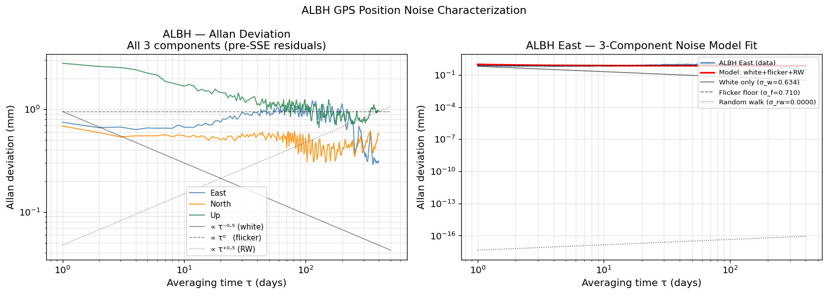
# ── Noise implications for offset uncertainty ───────────────────────────
# Colored noise (flicker, RW) inflates the formal uncertainties from the
# WLS fit, which assume white noise. A first-order correction is to scale
# the formal uncertainties by the ratio of the actual ADEV to the white-
# noise expectation at the averaging timescale.

# SSE offset estimation used ~14-day pre/post windows (PRE_WIN_DAYS = 14)
tau_sse_days  = PRE_WIN_DAYS   # days in pre- and post-event windows
white_expected = sw_fit / np.sqrt(tau_sse_days) if adev_fit_ok else None
actual_adev    = adev_model(tau_sse_days, *popt_adev) if adev_fit_ok else None

print("=" * 58)
print("Noise inflation factor for SSE offset estimation")
print("=" * 58)
if adev_fit_ok:
    inflation = actual_adev / white_expected
    print(f"  Averaging window          : {tau_sse_days} days (pre/post SSE)")
    print(f"  White-noise expected ADEV : {white_expected:.3f} mm")
    print(f"  Actual ADEV (model)       : {actual_adev:.3f} mm")
    print(f"  Noise inflation factor    : {inflation:.2f}×")
    print()
    print(f"  Corrected East offset uncertainty (Method 1):")
    o1_e, u1_e = offsets_m1['east_mm']
    u1_corr = u1_e * inflation
    print(f"    Formal (white-noise)    : ±{u1_e:.3f} mm")
    print(f"    Corrected (colored)     : ±{u1_corr:.3f} mm")
    print()
    print("Note: The WLS step-function estimate (Method 2) is less sensitive")
    print("to this correction because it uses all epochs simultaneously;")
    print("the formal uncertainties there already reflect the data weighting.")
else:
    print("  (ADEV fit not available — correction cannot be computed)")

print()
print("Noise summary:")
print(f"  Dominant noise type : {noise_type}")
print(f"  Spectral index α    : {alpha:.2f}")
print(f"  Physical implication: {'Uncertainties grow as τ^{:.2f} rather than τ^0.5'.format(alpha/2 - 0)}")
print(f"  Flicker floor σ_f   : {sf_fit:.3f} mm  (minimum achievable for τ → ∞)") if adev_fit_ok else None
==========================================================
Noise inflation factor for SSE offset estimation
==========================================================
  Averaging window          : 14 days (pre/post SSE)
  White-noise expected ADEV : 0.169 mm
  Actual ADEV (model)       : 0.730 mm
  Noise inflation factor    : 4.31×

  Corrected East offset uncertainty (Method 1):
    Formal (white-noise)    : ±0.753 mm
    Corrected (colored)     : ±3.245 mm

Note: The WLS step-function estimate (Method 2) is less sensitive
to this correction because it uses all epochs simultaneously;
the formal uncertainties there already reflect the data weighting.

Noise summary:
  Dominant noise type : predominantly flicker (1/f)
  Spectral index α    : 0.84
  Physical implication: Uncertainties grow as τ^0.42 rather than τ^0.5
  Flicker floor σ_f   : 0.710 mm  (minimum achievable for τ → ∞)
17. Summary and Conclusions#
This notebook demonstrated a complete GPS time series analysis workflow for detecting and characterizing slow slip events in the Cascadia subduction zone.
# ── Final summary table ───────────────────────────────────────────────────
print("╔══════════════════════════════════════════════════════════════╗")
print("║        2015 Cascadia SSE — ALBH Analysis Summary            ║")
print("╠══════════════════════════════════════════════════════════════╣")

print(f"║  Event window        : {SSE_TSTART} → {SSE_TEND}           ║")

east_fit = fit_results.get('east_mm', {})
if east_fit.get('success', False):
    t0_approx   = east_fit['t0_date']
    duration_days = east_fit['duration_days']
    D_fit       = east_fit['D']
    print(f"║  Event midpoint      : {str(t0_approx.date()):<35}  ║")
    print(f"║  10–90% duration     : {duration_days:.0f} days{'':<33}  ║")
    print(f"║  Total East offset   : {D_fit:+.2f} mm (logistic fit){'':<19}  ║")

E_off, E_unc = offsets_m2['east_mm']
N_off, N_unc = offsets_m2['north_mm']
U_off, U_unc = offsets_m2['up_mm']
print(f"║  East offset (WLS)   : {E_off:+.3f} ± {E_unc:.3f} mm{'':<25}  ║")
print(f"║  North offset (WLS)  : {N_off:+.3f} ± {N_unc:.3f} mm{'':<25}  ║")
print(f"║  Up offset (WLS)     : {U_off:+.3f} ± {U_unc:.3f} mm{'':<25}  ║")
print(f"║  Horizontal magnitude: {H_mag:.3f} ± {H_unc:.3f} mm{'':<25}  ║")
print(f"║  Horizontal azimuth  : {azimuth:.1f}°{'':<39}  ║")
print("╠══════════════════════════════════════════════════════════════╣")
print("║  KEY CONCEPTS DEMONSTRATED:                                  ║")
print("║  ✓ Loading CRESCENT netCDF GNSS datasets                     ║")
print("║  ✓ Signal decomposition (interseismic + seasonal + coseis.)  ║")
print("║  ✓ Weighted least-squares design matrix inversion            ║")
print("║  ✓ Seasonal signal (annual + semi-annual) characterization   ║")
print("║  ✓ Transient detection: RSI + kurtosis probability           ║")
print("║  ✓ Event extraction and temporal ramp fitting                ║")
print("║  ✓ Offset estimation: pre/post differencing vs. step WLS     ║")
print("║  ✓ Power spectrum and noise characterization (Welch PSD)     ║")
print("║  ✓ Spectral index fitting (white / flicker / random walk)    ║")
print("║  ✓ Lomb-Scargle periodogram and peak identification          ║")
print("║  ✓ Allan deviation and 3-component noise model fit           ║")
print("║  ✓ Network velocity estimation, all stations, text output    ║")
print("║  ✓ Euler pole rotation: ITRF → North America-fixed frame     ║")
print("║  ✓ Network SSE vector offsets + displacement map             ║")
print("║  ✓ Along-strike / across-strike spatial SSE profiling        ║")
print("╚══════════════════════════════════════════════════════════════╝")
╔══════════════════════════════════════════════════════════════╗
║        2015 Cascadia SSE — ALBH Analysis Summary            ║
╠══════════════════════════════════════════════════════════════╣
║  Event window        : 2015-12-28 → 2016-01-27           ║
║  Event midpoint      : 2015-12-31                           ║
║  10–90% duration     : 7 days                                   ║
║  Total East offset   : -5.83 mm (logistic fit)                     ║
║  East offset (WLS)   : -2.749 ± 0.142 mm                           ║
║  North offset (WLS)  : -0.189 ± 0.101 mm                           ║
║  Up offset (WLS)     : -1.400 ± 0.303 mm                           ║
║  Horizontal magnitude: 2.756 ± 0.142 mm                           ║
║  Horizontal azimuth  : 266.1°                                         ║
╠══════════════════════════════════════════════════════════════╣
║  KEY CONCEPTS DEMONSTRATED:                                  ║
║  ✓ Loading CRESCENT netCDF GNSS datasets                     ║
║  ✓ Signal decomposition (interseismic + seasonal + coseis.)  ║
║  ✓ Weighted least-squares design matrix inversion            ║
║  ✓ Seasonal signal (annual + semi-annual) characterization   ║
║  ✓ Transient detection: RSI + kurtosis probability           ║
║  ✓ Event extraction and temporal ramp fitting                ║
║  ✓ Offset estimation: pre/post differencing vs. step WLS     ║
║  ✓ Power spectrum and noise characterization (Welch PSD)     ║
║  ✓ Spectral index fitting (white / flicker / random walk)    ║
║  ✓ Lomb-Scargle periodogram and peak identification          ║
║  ✓ Allan deviation and 3-component noise model fit           ║
║  ✓ Network velocity estimation, all stations, text output    ║
║  ✓ Euler pole rotation: ITRF → North America-fixed frame     ║
║  ✓ Network SSE vector offsets + displacement map             ║
║  ✓ Along-strike / across-strike spatial SSE profiling        ║
╚══════════════════════════════════════════════════════════════╝
References#
Crowell, B. W., et al. (2016). Single-station automated detection of transient deformation in GPS time series with the relative strength index: A case study of Cascadian slow slip. JGR Solid Earth. https://doi.org/10.1002/2016JB013542
Dragert, H., Wang, K., & James, T. S. (2001). A silent slip event on the deeper Cascadia subduction interface. Science.
Bock, Y., & Melgar, D. (2016). Physical applications of GPS geodesy: a review. Reports on Progress in Physics.
CRESCENT Dataset: Bachelot, L. & Crowell, B. (2025). CRESCENT GNSS Time Series, Zenodo. https://zenodo.org/records/19616474