Making 3D fault geometries from cross-sections

This tutorial describes how to create complex 3D fault geometries from geologic map and cross-section data using QGIS, with custom plugins created specifically for this purpose. In this tutorial, we will use data (geologic mapping and cross-sections) from a 2018 paper on the Yakima Folds Province by Lydia Staisch.

The finished product will look something like this version visible in the 3d viewer here: http://rocksandwater.net/yfp_3d/

There are 3 steps to this process:

1. First is data preparation. This is pretty simple.

2. Then, we’ll georeference the cross-sections and digitize points on the faults in the cross-sections, so that we can see the fault geometries (in the cross-sections) in the QGIS map panel. We’ll also be able to view the cross-section images with any other 3D geospatial data in three dimensions using the Qgis2ThreeJS plugin, which will help a lot in understanding and quality-checking the fault geometries that we’re making.

3. Finally, we’ll draw contours based on the cross-section data and map patterns, and then mesh those to form fault surfaces.

Step 1: Data Preparation and Plugin Installation

Data Preparation

The first task is to gather the map and cross-section imagery. While the map was initially created in a GIS program, we don’t have easy access to it, and in general you won’t either. Screen captures will work fine, though the map will need to be georeferenced, which we won’t cover here.

The image below is a screen capture of the geologic map from Staisch et al. 2018. It was captured from the pdf using MacOS’ Preview application and exported as a .png file, then georeferenced using QGIS’s Georeferencer tool, and saved as a geotiff.

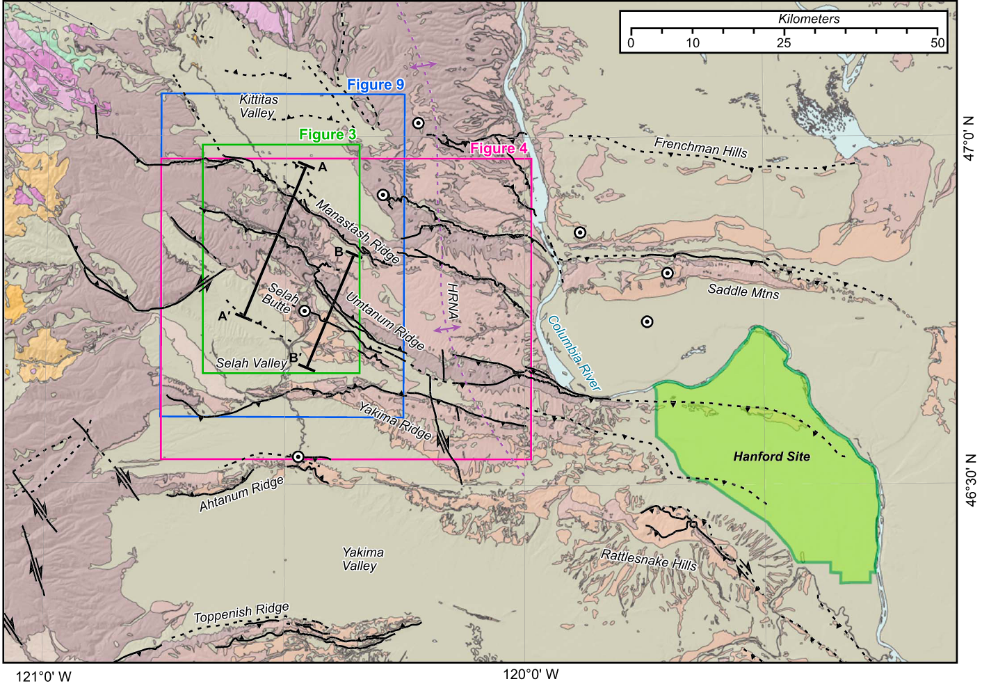Geologic Map of the Yakima Folds Province

Below that are two cross-sections, A-A’ and B-B’. These are just screen caps, without any other information.

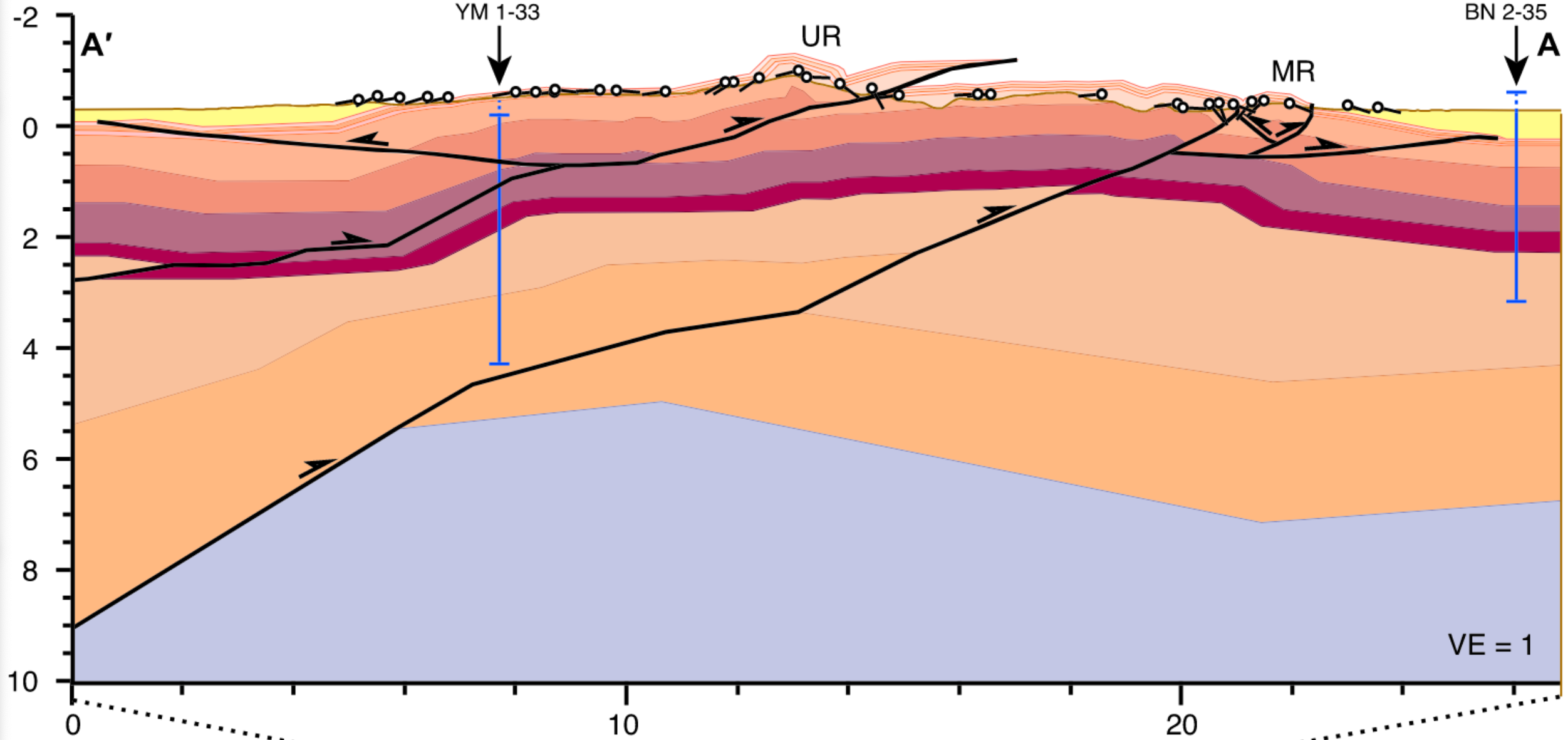Cross-Section A-A’

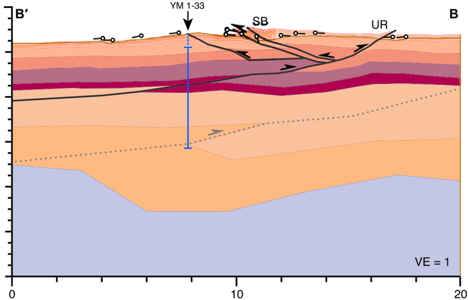Cross-Section B-B’

You can just save these to your hard drive and get to work georeferencing.

update, 8 August 2025

I’ve made the georeferenced tif available here, for the sake of expediency:

staisch_et_al_2018_map.tif

Plugin Installation

You need to install 3 plugins. The easiest way is to download the latest .zip from the release page of the following repo:

QGIS2ThreeJS (this version has capabilities to view cross-sections compared to the original plugin)

Cross-Section Digitizer

Contours2Mesh

Then, open the ‘Manage and Install Plugins…’ window from the ‘Plugins’ menu, and click on ‘Install from ZIP’ on the left side, and install each.

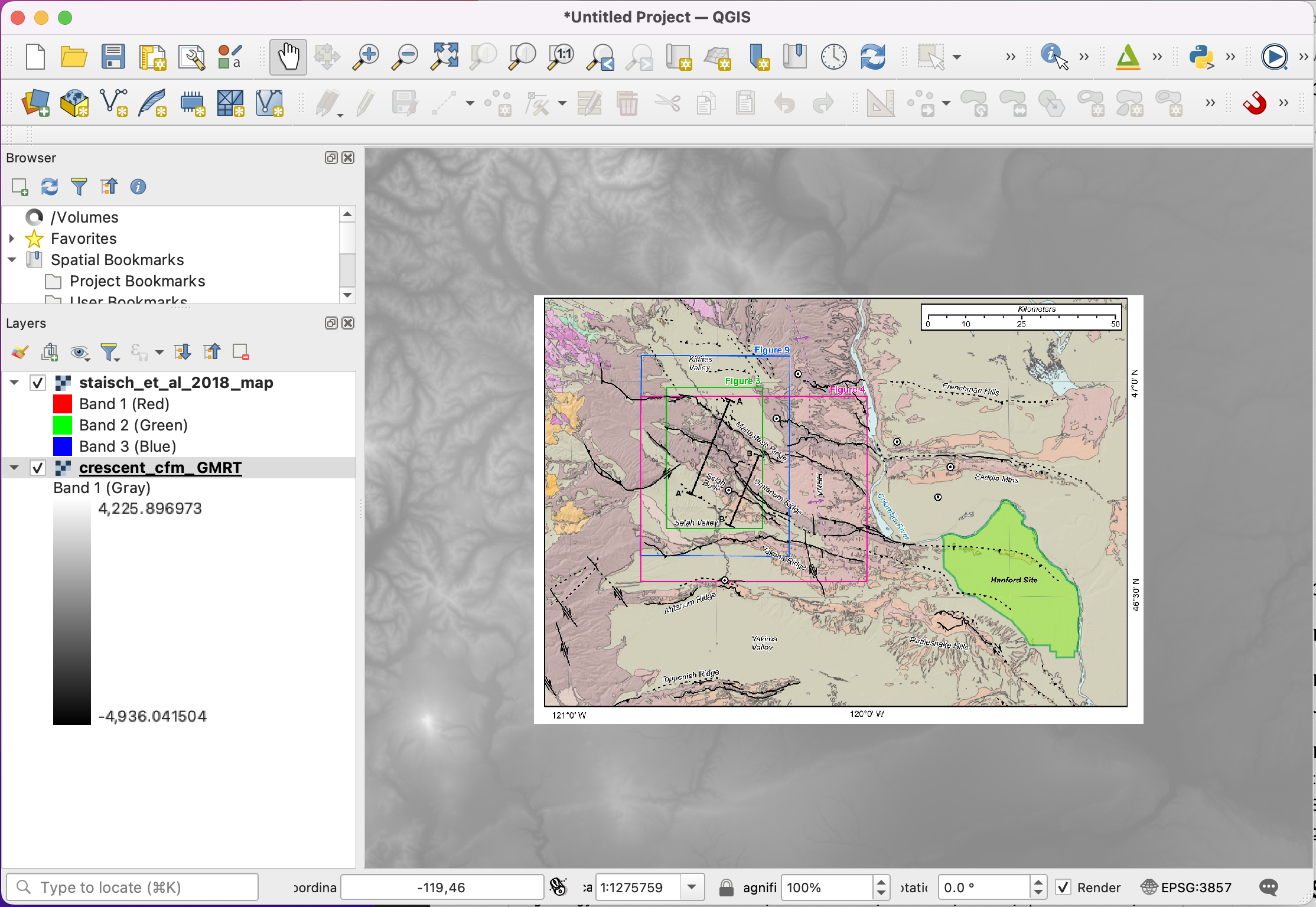
Loading the data

Now that we have the data, first we’ll load the map into QGIS. We’ll also have a DEM to get the elevations of the points on the surface trace. This is something that you can find for yourself; just make sure the elevations are in meters. It’s probably also important for the [CRS] of the DEM to be in EPSG:4326 (WGS84). However, we don’t need to have the QGIS map in EPGS:4326, because at this latitude, there is substantial distortion, so I’m changing it to EPSG:3857, which is a nice projected coordinate system for many tasks.

Step 2: Georeferencing the cross-section and digitizing the fault data

Georeferencing the Cross-Sections

The next step is to open the Cross-Section Digitizer plugin. It will probably load as a panel on the right side of the QGIS main window. Depending on your screen real estate and preferences, you can leave it here or detach it.

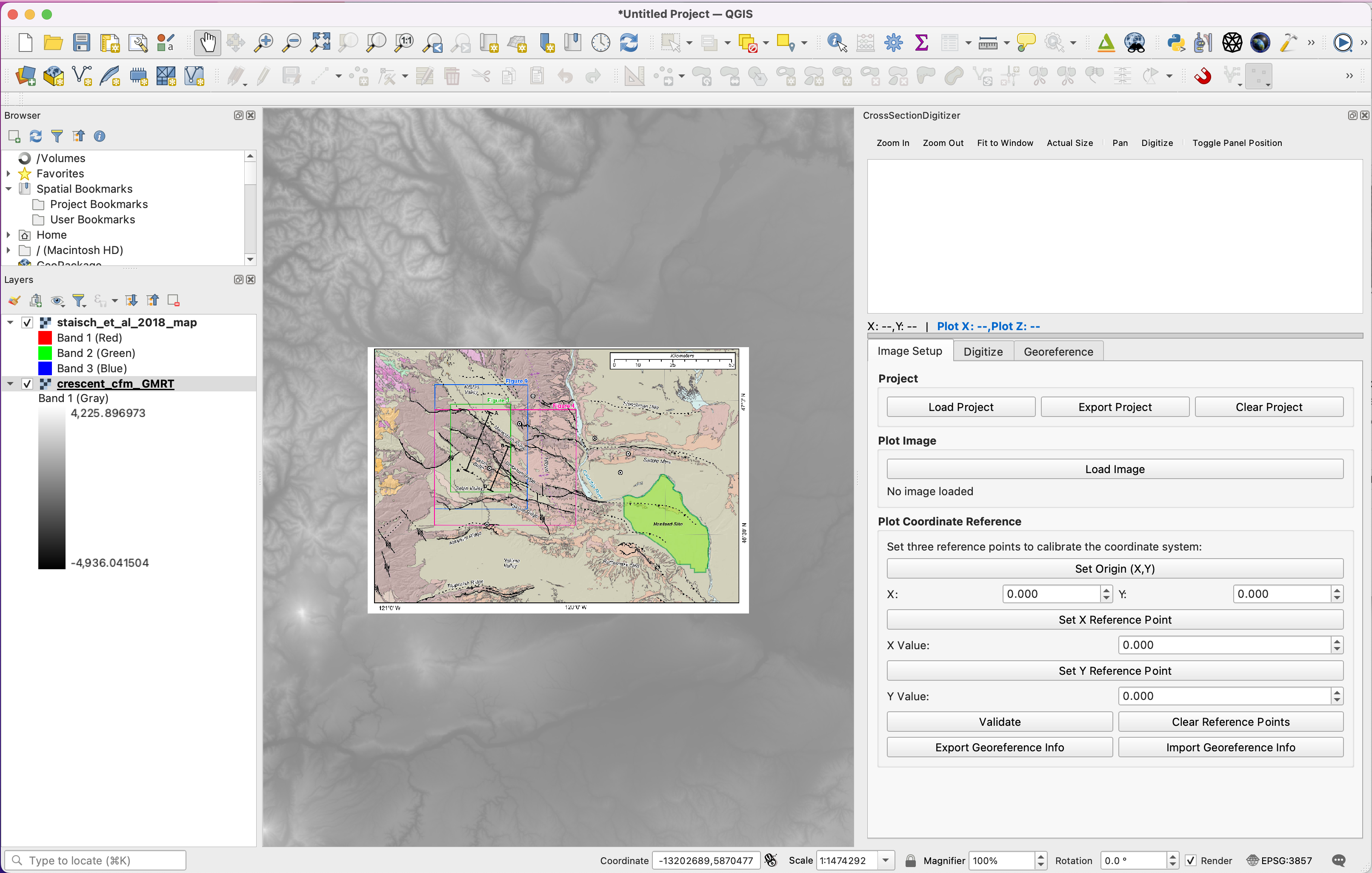
Now, we want to digitize the A-A’ cross-section, so click on the ‘Load Image’ button under the headline ‘Plot Image’, and select staisch_2018_a-aprime.png. It will display in the window at the top.

Setting up plot (cross-section) coordinates

The next step is to make a Plot Coordinate Reference system, which is based on the plot axes in the cross-section picture; this lets the computer transfer a point from the computer’s pixel coordinate system into the geographic space defined by the cross-section. (Note that Staisch was characteristically thorough by including both X and Z coordinate axes on the figure; many authors neglect the X axis, which makes it more difficult: you would have to find that information from the map or estimate it somehow.)

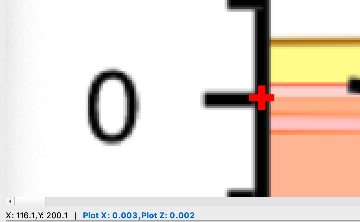
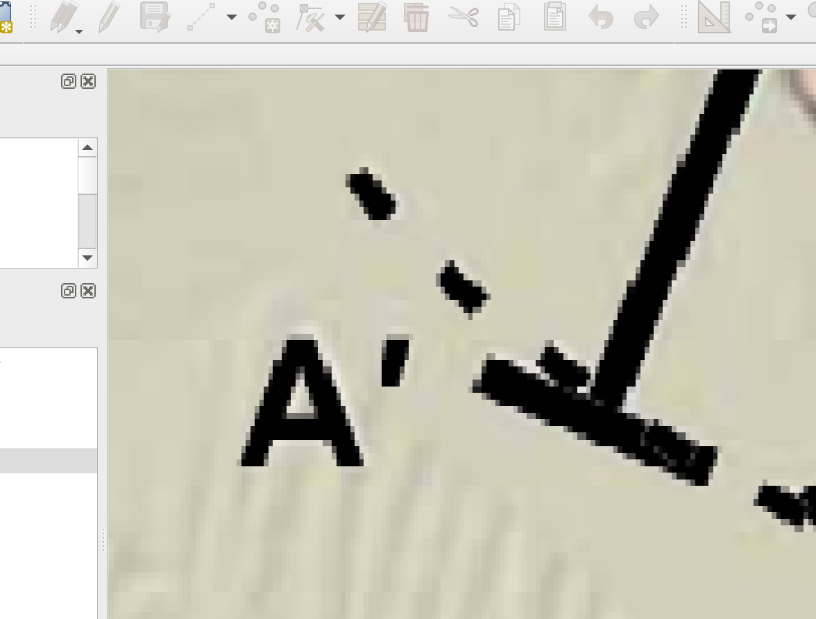
Click on the ‘Set Origin (X,Y)’ button, then move your mouse up to the image. You’ll see a little cross for the cursor. Then, pick a handy point such as the lower left corner of the cross-section, and click as accurately as possible on it. Note that you can zoom with the mouse wheel, and click ‘Pan’ in the menu bar on the top to move the image around and ‘Digitize’ to go back to clicking points.

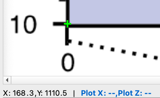
I clicked here on the lower left point. Then, I fill in the X and Y fields with the cross-section values. The X value is 0 (km), but the Y value is 10; this is depth, but we want a positive-up system so I’ll put -10 in the box.

Then, I did the same for the X reference point–I clicked at the ‘20 km’ tick. Note that the Y/Z value isn’t used, so you just have to get the X value right. Then fill in the box with 20. Then do the same for the Y value, making sure to make the value have the opposite sign as in the cross-section if the values are depths. 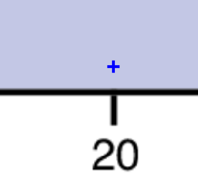X value

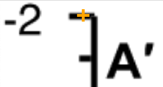Y value

Once you have the 3 point set, that is enough to make a coordinate transformation. Just click ‘Validate.’ If the values are all filled in (not to say correct), you’ll get a happy message. Also, the blue ‘Plot X’ and ‘Plot Z’ values will be filled in as you move your mouse around the cross-section, which is useful when digitizing points.

Georeferencing the cross-section

Now that we have a transformation between image to plot coordinates, we need to make another transformation from plot to geospatial coordinates.

Click on the ‘Georeference’ tab below the plot. We’re going to click on two points on the cross-section that we can tie to two points in the map. (Note that if you don’t have the map loaded in QGIS but know the start and end points of the cross-section, you can just enter that inforamation instead of using the map window.)

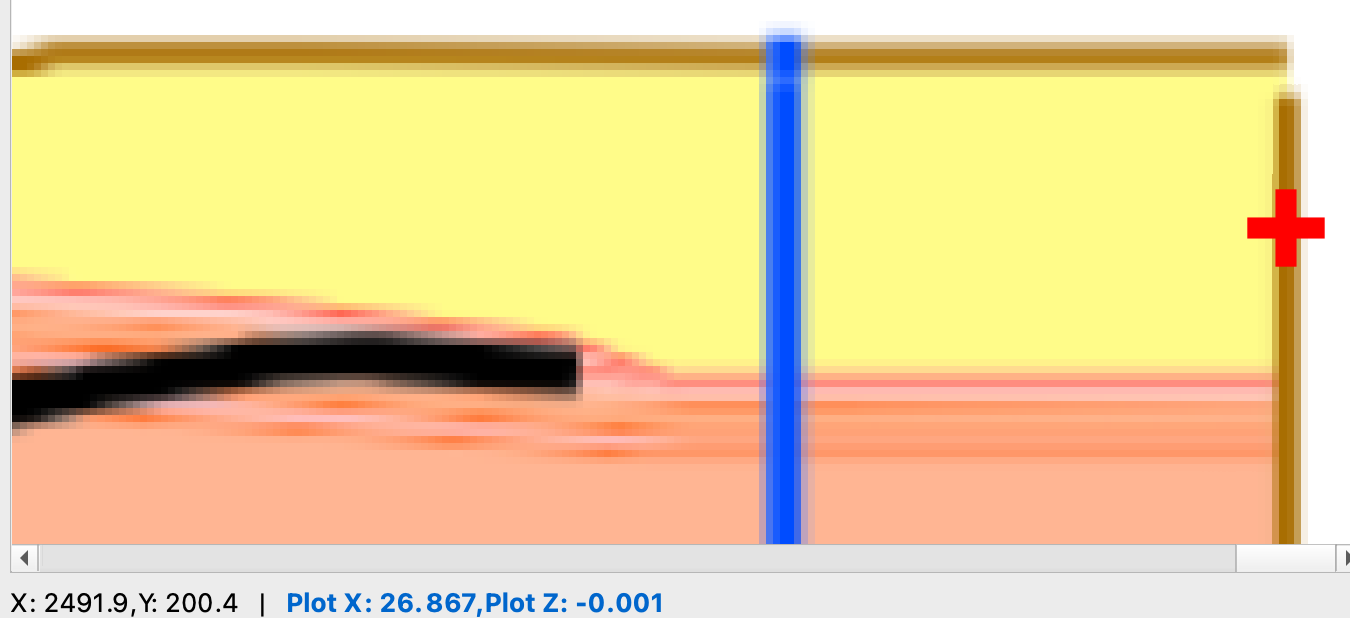
Click on ‘Click Start Point on Plot’ and then click the start point on the plot. This should be one end of the plot (I went left) in terms of the X value, since that will be tied to the end point of the cross-section on the map. The Z value can be anything, but pay attention to it. In my click the Z value was 0.002, which corresponds to an elevation of 2 m.

Start point

Then, do the same for the end point. End point

Now, click on the ‘Click on Map for Start Point’, and click on the end of the cross-section at A’ since that corresponds to the Start Point on the plot (if the map isn’t in WGS84 coordinates you’ll get a friendly message which you can ignore). This will fill in the longitude and latitude of the point in the boxes. However, it won’t fill in the Elevation value so you’ll get that from the Z value above. We had ‘Z=0.002’ (in km) which is 2 m, so we’ll enter 2.0 for the elevation.

Then do the same for the map end point. I had a value of Z=-0.001 so I will use -1.0 m for the elevation.

Now the georeferencing is done! You can click on ‘Create Georeferenced Polygon’ and a new layer will be created in the QGIS map window corresponding to the outline of the entire (georeferenced) cross-section image (not just plot–the axes and any extraneous pixels will be there).

Saving the work

This was a bit of tedious work, and we don’t want to have to re-do it every time we want to digitize more points (which we’re about to start doing) so we can save it all now. Go back to the ‘Image Setup’ menu and click on ‘Export Project’, and you can save a JSON file that has all the information necessary to replicate what we’ve done so far, as well as any further digitization.

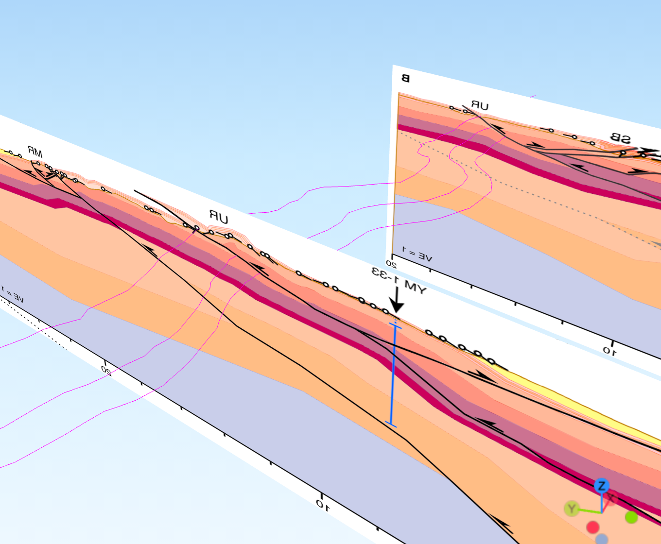
Viewing the cross-section in 3D

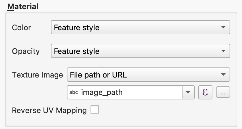
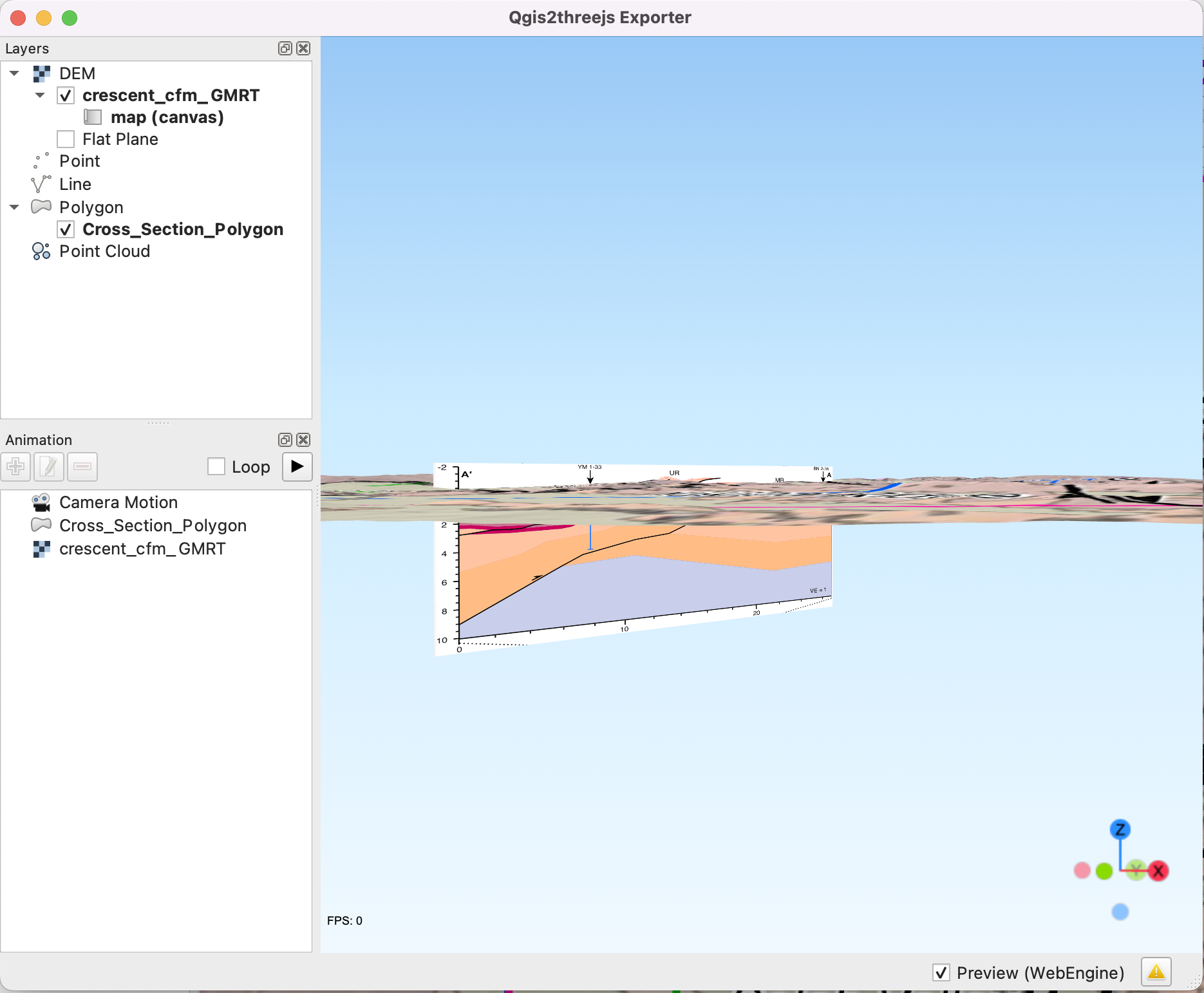
The next thing to do is to see the cross-section vertically, in 3d, in all its glory. First, open the Qgis2threejs Exporter. Then, click on the box to show the polygon, which is probably called ‘Cross_Section_Polygon’. This will show the polygon with the color it has in the map window. In order to show the image, right click on the item in the menu, and click on the little triangle next to the blank field for the ‘Texture Image’ field. Then, select ‘image_path’ which is an attribute of the polygon layer, which contains the location of the cross-section image (not the polygon) on your computer. Then hit ‘Apply’ and check to see that it’s oriented correctly. If it’s backwards (so that A on the cross-section matches with A’ on the map) then click the ‘Reverse UV Mapping’ box.

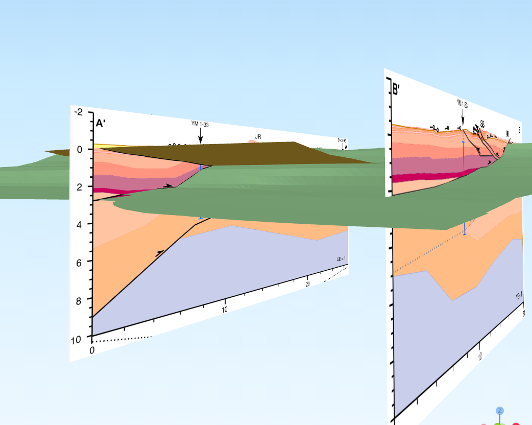
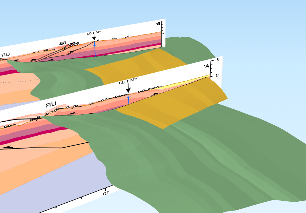
If everything went well, you should be able to see the cross-section like this:

Digitizing the fault data

Now, we’re going to digitize and georeference the fault data from the cross-section, so that we can see it in the map window and use it as a guide when making the contours.

The map and cross-sections show complex fault geometries. Both of the main faults, the Umtanum fault and the Manastash fault, have variable dips, as well as splays.

Though it is possible to build geometries for all of these faults, we’ll limit ourselves for now to the Umtanum Fault (which daylights in both sections) as well as the backthrust shown in Section A-A’ (which is blind). This will let us learn how to deal with complex 3D fault geometries, and how to make faults merge at depth, without getting too bogged down.

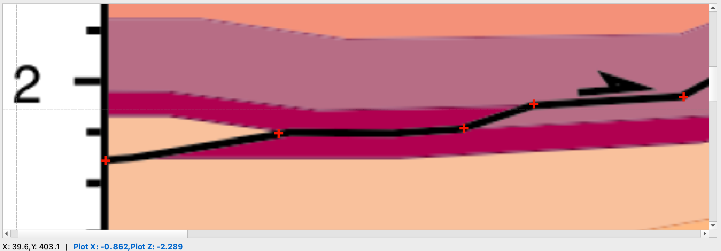
To do this, we’ll go back to the Cross-Section Digitizer plugin; this time, we’ll use the ‘Digitize’ tab. First, we need to name the new Data Series, so type ‘Umtanum A’ in the box, and hit ‘New Series’. Then, we’ll start clicking on important points on the fault; these are basically the hinge points, where the fault dip changes. Note that when you use a mouse, you can zoom in and out with the wheel; it’s much, much easier with a mouse than the trackpad. Click ‘Start Digitizing Points’ and just go for it. When you click, points will be added to the list. You can delete them if you click in the wrong place.

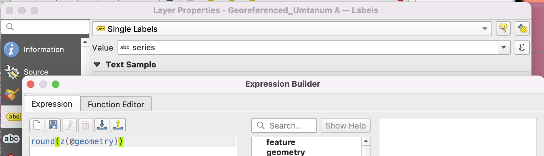
Then, once you’re satisfied, you can go to the ‘Georeference’ tab in the plugin window, and click ‘Georeference Digitized Points’. This uses the information already provided to map coordinates from cross-section space to geographic space, so we don’t have to do that again. Instead, the points will appear in the map window, as a new point layer. To make the useful, we’ll label the points by their elevation (z value) so that we can see them in the map. Go to the ‘Properties’ for the layer, hit ‘Single Labels’, click on the ‘Expression’ button (the curly E) and then enter round(z(@geometry)), which fetches and formats the elevations from the points’ geometries. Format the text so you can easily read on your screen.

It’s also a good time to save the work. You can save the project again as discussed above, and it will preserve the points clicked. However the georeferenced points in the map window won’t be saved. They can be trivially exported again by hitting the Georeference Digitize Points button, but the points layer can also be saved from the QGIS layers menu.

Now we can do the same for the Umtanum backthrust. Go to the ‘Digitize’ tab in the plugin, type a new series name, and get to it.

Interlude: Doing the same for B-B’

In this demo, we have a second cross-section, B-B’. The same process (load the cross-section, make the coordinate transform, georeference it, digitize the fault points) needs to be done. Since the process is identical, it won’t be explained in detail here. Save the work when you’re done.

The Umtanum backthrust evident in A-A’ is not the same backthrust in B-B’. Therefore the fault stops somewhere in between the section lines. So in B-B’, we only have one fault to digitize.

Another helpful thing to do with the Umtanum fault in both sections is to write down the elevation values of the points in each section, then go to the other section and click on points on the fault with that same elevation (unless there is already one really close). This ensures that both sections have points at the same elevations which makes drawing contours much easier. You can only have one cross-section loaded in the digitizer each time so you’ll have to save and re-open.

Step 3: Drawing contours

Now we have the points for the Umtanum fault loaded in the map for both cross-sections, and they are labeled visibly by their elevations (for clarity, un-click the Umtanum Backthrust box so you can’t see it).

Make the contour file

We’ll first make a file to store the contours in. Make a new layer by clicking through ‘Layer -> Create Layer -> New Temporary Scratch Layer’ and then give the layer a name that you would like. Then make the geometry ‘LineString’ and click the ‘Include Z Dimension’ box. Then make a new field called ‘elev’ with the type ‘Decimal (double)’, and then one called ‘name’ with type ‘Text (string)’. Then hit ‘OK’.

Note that this file is just stored in RAM or in a temp directory, depending on your operating system, and it may or may not be stored if you quit QGIS without saving it. However we’ll make at least one feature (contour) before saving so that we’re sure that it gets saved correctly–sometimes saving an empty geojson file doesn’t work super well because the attribute fields get lost.

Draw contours

The first contour we’ll draw is the map trace. It’s already mapped although it becomes inferred just before the B-B’ section but we’ll continue it.

Click on the ‘Add Line Feature’ button from the digitizing menu bar and go to work. If you don’t know how to do this, please look for resources online–they are abundant. When you’re done clicking, leave the ‘elev’ field blank and then name it something like ‘umtanum_trace’. Then hit the ‘Save Layer Edits’ button (the floppy disk) even though it’s still a temporary file and your computer probably doesn’t even have a floppy disk drive.

If the default symbology is hard to read, then change it to something more visible.

Also, pay attention to the direction you click when you’re digitizing. I tend to digitize points from left to right, because I’m right-handed and that’s how I draw. These all either need to be drawn consistently, or they can be changed after digitizing with the ‘Reverse Line’ button in the ‘Advanced Digitizing’ menu. If you use a symbology that indicates the point direction (such as one of the fault symbologies from here) then you can see whether the points are all in a consistent order.

Add elevations from DEM to trace

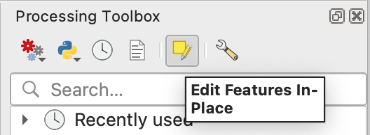
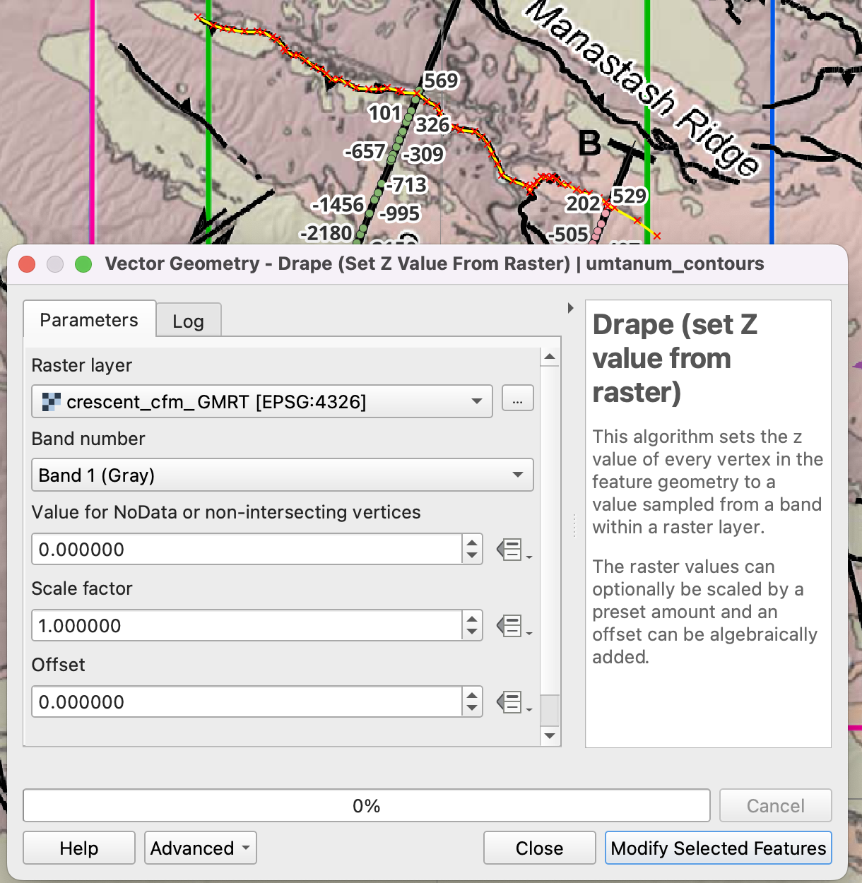
Now, open the Processing Toolbox, and then click on the yellow button on the top that is the ‘Edit Features In-Place’ button.

Then, use the ‘Select Features’ button to select the fault trace.

Then, go back to the Processing Toolbox and type ‘drape’ in the Search bar. Select the DEM that you want to use from the Raster field (it will appear if it’s loaded, otherwise you’ll have to dig one up from your hard drive or a floppy disk). As long as the feature is selected, there should be a ‘Modify Selected Features’ button in the lower right. Click it.

Then, de-select that feature.

Making other contours

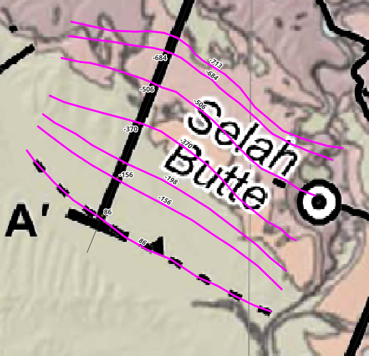
Most of the time, the contours are lines of constant elevation. To make these, draw your own contour lines that pass through the cross-sections where they are indicated by the digitized points or where your geologic spidey sense tells you to.

After you finish each feature, you can fill in the ‘elev’ field with the elevation, and then name the feature something similar; these steps themselves are not absolutely necessary but sure make things easier. Then, add a label to the features in the map, using the ‘elev’ field, so you can see the value of the contours while you are working, which will definitely make things easier.

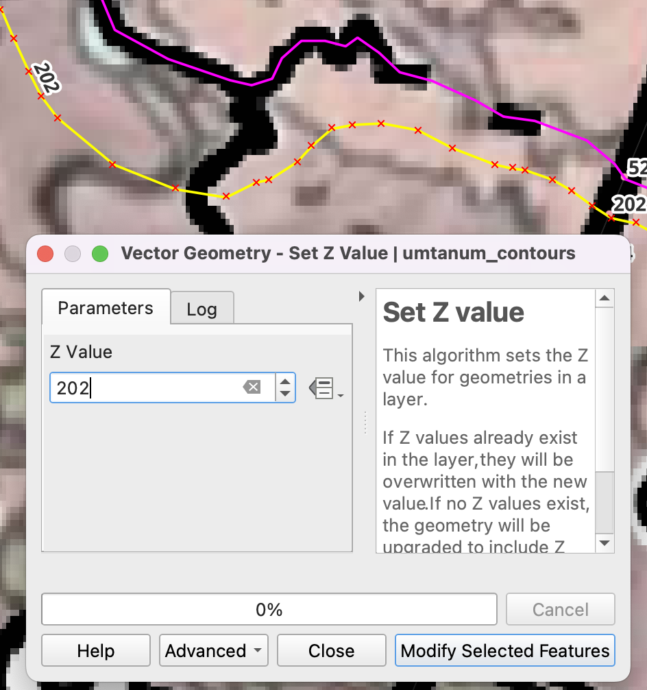
After you draw a contour, then assign an elevation value to all of the vertices in it. Unlike using the ‘Drape’ tool earlier (which assigns a value to each vertex based on the closest DEM value), we’ll assign a single value to all vertices. Select the contour, then search for the ‘Set Z value’ in the Processing toolbox. Then give it the right elevation, and hit ‘Modify Selected Features’.

Once you’ve done this for at least one feature, it is wise to save the contours to a geojson file.

As long as the contours have Z values, you can also load them up into the Qgis2threejs plugin and see them plotted with the cross-sections. Note that if the map is zoomed in too far (in the main QGIS window) then sometimes the points are given a zero elevation. Don’t ask me why.

Once you’re done, you’ll have a lot of contours. As is evident based on the cross-sections, there are subtle differences in structure in the cross-sections that are manifest in non-parallel contour lines. Thus, we can’t simply project the trace down to depth like we could with less information.

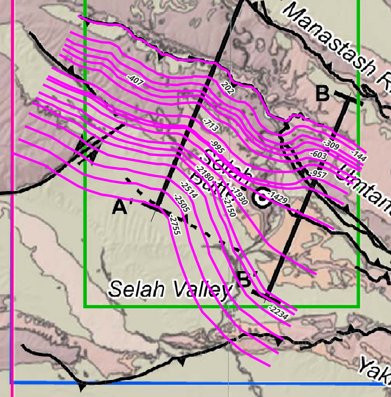
Specifically, it’s clear that the Umtanum fault in the B-B’ cross-section is a bit steeper up top but then flattens out quite a bit between 1-2 km depth, but the A-A’ cross-section shows a more planar fault.

Mesh the fault

Now, it’s time to mesh the fault, making a 3D surface composed of triangles sharing edges.

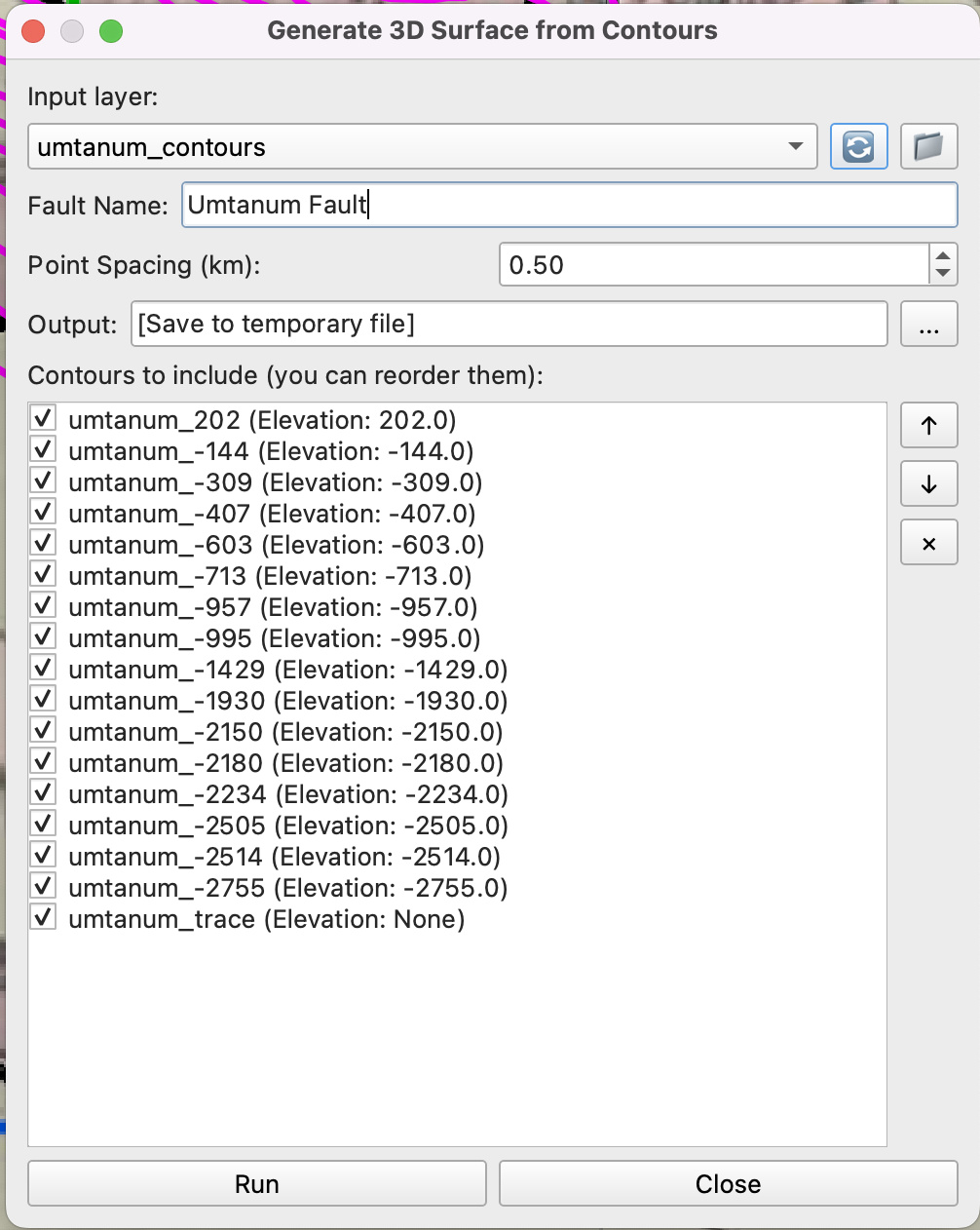
Click on the ‘Generate 3D Surface from Contours’ plugin. Select the ‘umtanum_contours’ layer, then name the fault. Change the point spacing if you want (this is the approximate edge length of the triangles). The contours should show up in the order specified by the ‘elev’ field, but you should check based on the names to make sure it’s correct. Note that this time, the trace (Elevation: None) appeared at the bottom of the list. It is the top, so it needs to be moved to the top of the list. There are buttons to move items up and down, and to remove items from the list, on the right. There are also check boxes that you can uncheck to remove contours from the mesh, without removing them from the list (if that’s what you want to do). By default, the plugin makes a temporary file that is loaded into the QGIS window, but you can also save to a file by specifying something here. Hit ‘Run’ when you’re satisfied.

We’ve got a mesh! If you like it, close the plugin.

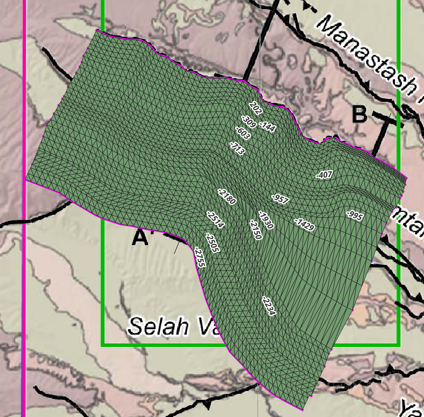
You can also see the mesh in the Qgis2threejs window:

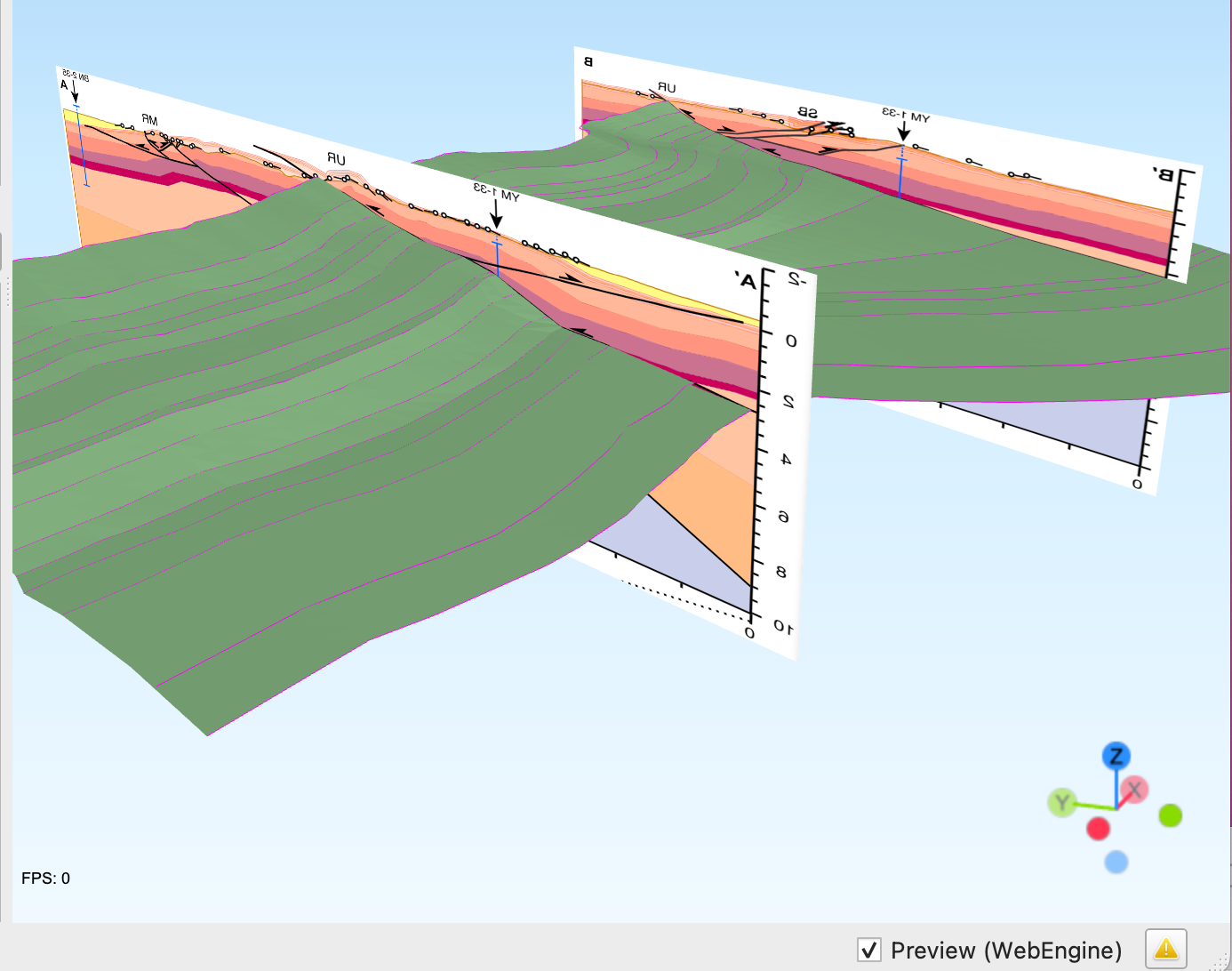
If it comes up clear when you load it, you have to clear the ‘Texture image’ field and hit ‘Ok’. Not sure why…

This is your chance to quality control your contours. Now, it is much easier to see the 3D geometry of the fault. If there are things that you don’t like–maybe it doesn’t match the cross-sections or other data sufficiently, or maybe there are some weird bits in between the sections, or whatever, go back and move the vertices on your contours, or add/subtract contours, and re-mesh until you’re happy.

You can also start making and visualizing the mesh once you have at least 2 contours drawn, just in case you’re curious or want to QC before you’re finished.

Contour and mesh the backthrust

Now, it’s time to draw the backthrust. This fault is inferred on the surface with a relatively short trace, only in section A-A’. It merges with the Umtanum fault at -713 m in the cross-section.

In order to make it merge seamlessly across its length, make the branch line at that depth for its whole breadth. The easiest way to do that is by copying the -713 m contour from the Umtanum fault and then renaming it. Then filter the layer by name (use a filter like "name" LIKE 'umtanum_backthrust%' so only the backthrust is visible. After you have all of the contours drawn, trim along strike.

Then, mesh the backthrust with the plugin, and look at it in 2D and 3D to assess.

If you’re satisfied with the geometries, you’re good to go! Save the files to your format of preference, and move along with your life!

References

Staisch, L., Blakely, R., Kelsey, H., Styron, R., and Sherrod, B., 2018, Miocene to present-day deformation rates in central Washington, USA, revealed by stream profiles, potential-field geophysics, and structural geology of the Yakima folds, Tectonics, vol. 37, no. 6, p. 1750-1770, doi: 10.1029/2017TC004916